Well in Shape - The Right Data Type in R, Stata, and SPSS

R
Statistics & Methods

24. November 2017

Jessica Gerhard

Team AI Academy

Once the dataset has been imported into the desired statistical program, there are often a few pitfalls before you can begin applying the method. This is often because the variables are not assigned the correct type. For example, if values that are actually numbers are stored as strings (character strings), measures of central tendency for the distribution cannot be calculated. Therefore, after importing the data, the next step should be to check the data type of the variables, which is usually assigned automatically by the statistical software—and not always correctly.

Dataset

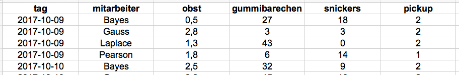
In the previous post, the data used was briefly introduced. It involves the recording of candy consumption by four STATWORX employees, whose real names have been replaced by their respective favorite statisticians. The head of the data is depicted below.

Data Types

In computer science, there are countless data types, primarily identified by their storage requirements. The enumeration of variable types is presented here in a simplified manner. Generally, variables can be qualitative as strings (character strings) or quantitative in numerical form. The latter can be further divided into integers and decimal numbers.

A special case of strings is the factor. This is an ordinal variable that has only a limited number of expressions. Each expression is represented as a numerical value and is assigned value labels. An example is the question about satisfaction with a product, where numbers 1 to 5 express satisfaction from "very dissatisfied" to "very satisfied."

Furthermore, it is important to distinguish the level of measurement of data. Data can be nominal, meaning without order, like gender, or ordinal, meaning ordered and thus having a fixed sequence, such as when using age groups. Other levels of measurement include the interval scale and the ratio scale. On the ratio scale, equal intervals on the scale represent equal differences. The difference between the value 10 and 20 indicates the same deviation as the difference between 30 and 40. Additionally, there is a natural zero point. An example of this is the measure of length. On the interval scale, there are also equal distances between the individual expressions, but there is no absolute zero point. A common example of this is temperature measurement in degrees Celsius.

Scale	Requirement	Example	Expressions
nominal	Difference	Gender	male, female
ordinal	Order	Candy consumption	none, little, a lot
Interval	Equal intervals	Degrees Celsius	30, 43
Ratio	Natural zero point	Meter measurement	0, 1.00, 1.11, …

In the case of strings, there can be internal types within the statistical software that classify the character string more specifically, such as a date format.

R

The structure of the data can be queried in R with str(). For the candy dataset, we obtain the following result:

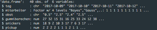
The type of individual variables (or vectors) can be queried with class(). It turns out that most types have already been recognized correctly. In general, any data types can be assigned with functions like as.datatype(), for example, as.numeric() or as.character().

The employee variable has only four expressions. R has recognized this and automatically coded the variable as a factor with values 1 to 4 and named the expressions “Bayes,” “Gauss,” etc. This helps save memory space. The reason the variable is automatically converted into a factor is that the stringsAsFactors option is automatically set to TRUE in data.frame.

The four variables regarding candy consumption have all been correctly identified as numeric values. However, what is not immediately clear is that the PickUp variable does not indicate how many bars are consumed per day, but rather which type the employee prefers. The value 1 should stand for the type “Choco,” 2 for “Choco & Caramel,” and 3 for “Choco & Milk.” The goal is a factor variable, as is also the case with the employees. The implementation is found in the code box below. Depending on whether the factor has ordinal values or not, the factor() or ordered() function can be used. Since the types have no order, the factor() function is used here.

The fruit variable is supposed to represent the number of pieces of fruit eaten, accurate to one-tenth. Unfortunately, it has been recognized as a string. This is often due to the decimal separator. Additionally, the problem can arise if the variable contains strings like “no information.”

Lastly, there is the date variable. One option for converting common date formats is the as.Date() function. The structure should be passed with the format argument. In the code box below, the conversion to the date format is shown. However, there are many other, more sophisticated ways to work with date formats in R, such as the lubridate package.

# Erstellen eines (ungeordneten) Faktors aus der PickUp-Variable 
sweets$pickup <- factor(sweets$pickup, 
levels = c(1, 2, 3), 
labels = c("Choco", "Choco & Caramel", "Choco & Milch")) 

# Umwandlung der Obst-Variable ins Zahlenformat 
sweets$obst <- as.numeric(sweets$obst) 

# Umwandlung der Tag-Variable ins Datumsformat 
sweets$tag <- as.Date(sweets$tag, format ="%Y-%m-%d")

After adjusting the data types, another look at the data shows that all variables now have the desired type.

Stata

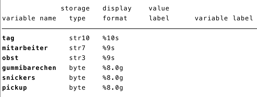
In Stata, a distinction is generally made between storage type and display format. The former indicates how much space the variable occupies in memory. It can also be determined whether it is a string (="str"; number at the end indicates the length) or numeric values (="byte", "float", "long", "double"). The structure of the variables can be viewed using the describe command.

Let's first address the PickUp variable, which was also read as numeric here but should be defined as a factor. First, a label must be defined, independent of the variable. This can then be applied to one or multiple variables. In the code box below, a label is first defined using the label define command, which is then applied to the variable with the label values command.

At first, it may seem a bit cumbersome to define and assign labels separately; however, there are often labels that are used frequently, such as naming the values 0 and 1 as "no" and "yes," or naming a satisfaction scale. By the way, the numeric values of an already labeled variable can be viewed with the nolabel option in the tabulate command.

Next, the fruit variable should be converted from a string to a numeric format. This is done in Stata with the destring command. The tostring command works in the opposite direction, converting from numeric format to string. With both commands, a new variable must be defined using the generate option. The reason the variable type was incorrectly recognized is the comma as the decimal separator (instead of a period). Therefore, the dpcomma option must be specified, which defines the comma as the decimal separator.

The date should be converted to the appropriate type if it is important for the analysis, such as in time series analysis. Here, too, a new variable must be created that displays the day in date format. As in R, the format in which the date is present must be specified after the variable name. The resulting variable is now defined in Stata's own format. The format command must then be used to select the structure in which the date will be displayed. For example, "%td" represents the display of the date without a time indication.

The employee variable is not automatically stored as a factor in Stata, unlike in R. It is stored as a string, which does not necessarily need to be changed. However, the transformation is shown below and can be helpful if you want to convert the variable for memory space reasons.

For this, the encode command can be used. With the label() option, the newly created numeric variable is immediately assigned the label.

* Definition der PickUp-Variable als Faktor 
label define chocolabel 1 "Choco" 2 "Choco & Caramel" 3 "Choco & Milch" 
label values pickup chocolabel 

* Umwandlung der Obst-Variable ins Zahlenformat 
destring obst, generate(obst_destring) 

* Umwandlung der Tag-Variable ins Datumsformat 
gen tag_date = date(tag, "YMD") 
format tag_date %td 

* Definition der Mitarbeiter-Variable als Faktor 
encode mitarbeiter, gen(mitarbeiter_faktor) label()

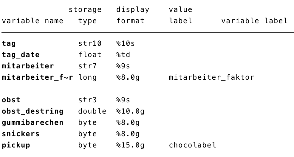
Nach Ausführung der Befehle wagen wir erneut einen Blick auf die Struktur der Daten. Im Vergleich zum Resultat in R, wurden in Stata viele neue Variable generiert. Selbstverständlich können die ursprünglichen Variablen auch entfernt werden. In R und auch SPSS ist es generell leichter bestehende Variablen zu überschreiben als in Stata. Das ermöglicht einen besseren Überblick über die Daten, kann jedoch auch gefährlich werden, wenn Variablen unabsichtlich überschrieben werden.

SPSS

Next, the adjustment of the data type in SPSS is introduced. The variable view is well-suited for examining the basic properties of the data. For us, the "Type" column is of interest here. This indicates whether it is a string, numeric values, or a date, for example. The level of measurement is displayed in a separate column.

Changes can also be made manually via the variable view. However, this can more easily lead to errors, and we want to introduce the SPSS syntax here. This way, changes can also be applied to multiple variables simultaneously. First, as before, let's look at the structure of the imported data:

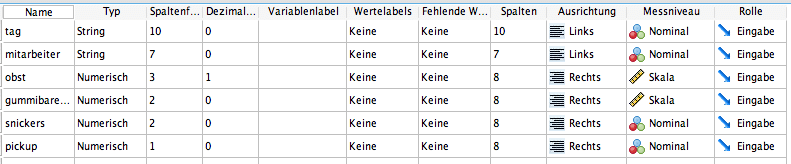
Once again, the date variable is not recognized in the intended type. Additionally, the Pickup variable should be defined as a labeled factor. The fruit variable with decimal values generally does not pose a problem because SPSS recognizes both periods and commas as decimal separators. For this reason, the variable is automatically assigned a decimal place.

Let's start with adjusting the PickUp variable. The VALUE LABELS command assigns a label to the numeric values. In SPSS's data view, you can switch between displaying numeric and labeled values using the "Value Labels" button. No further adjustments need to be made for the variable.

To convert the date variable into the appropriate format, a new variable must first be created with the NUMBER command. After the variable to be transformed, the order of the date is expected as the second argument. However, a direct conversion is also possible with the ALTER TYPE command. More information about the date type can be found here.

Additionally, it is shown how the string variable "Mitarbeiter" can be transformed into a factor. In this example, the user gains no advantage other than reduced memory space, but if it is a variable with an ordinal level of measurement, this conversion must be performed. The AUTORECODE command conveniently converts the string variable into a labeled numeric factor. The numbering is done alphabetically. This is not a problem here, but with a factor with an ordinal level of measurement, it can become a pitfall if the numbering is done automatically. The (unfortunately) simplest way to deal with this is to restructure all values individually into numeric sizes using the RECODE command and label them with the already familiar command. For this reason, the code box also illustrates how strings can be converted into factors with any expressions/any order.

In general, the variable type can be changed with the ALTER TYPE command. After the adjustments, we look again at the variable types in the variable view.

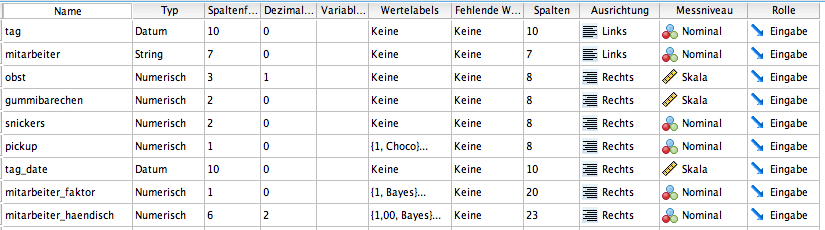
Both the newly created variable "tage_date" and the transformed day variable are now in date format. Two factors have been created from the string employee variable. One of them can be generated very easily (with AUTORECODE), while the creation of the second is more complex. However, the result of both is very similar: both have a numeric type as well as value labels. Labels are also now displayed for the PickUp variable.

* Definition der PickUp-Variable als Faktor 
VALUE LABELS pickup 1 "Choco" 2 "Choco & Caramel" 3 "Choco & Milch". 
EXECUTE. 

* Umwandlung der Obst-Variable ins Zahlenformat nicht notwendig, Komma automatisch als Dezimaltrenner erkannt. 

* Umwandlung der Tag-Variable ins Datumsformat 
COMPUTE tag_date=NUMBER(tag, SDATE10). 
FORMATS tag_date (SDATE10). 
EXECUTE. 

* Oder direkte Transformation des Datums:  
ALTER TYPE tag (SDATE10). 

* Definition der Mitarbeiter-Variable als Faktor 
AUTORECODE mitarbeiter /INTO mitarbeiter_faktor. 

* Mit beliebiger Nummerierung der Mitarbeiter-Variable 
RECODE mitarbeiter (CONVERT) ("Bayes" = 1) ("Pearson" = 2) ("Laplace" = 3) ("Gauss" = 4) INTO mitarbeiter_haendisch. 
VALUE LABELS mitarbeiter_haendisch 1 "Bayes" 2 "Pearson" 3 "Laplace" 4 "Gauss". 
EXECUTE.

Summary

This blog post attempts to highlight the most common issues related to data types in R, Stata, and SPSS. It becomes apparent that the same step in data preparation, namely adjusting the variable type, is implemented completely differently in the various software programs. Unfortunately, the transformation between types within a statistical program is often not intuitively understandable.