The helfRlein package – A collection of useful functions


We at statworx work a lot with R and often use the same little helper functions within our projects. These functions ease our daily work life by reducing repetitive code parts or by creating overviews of our projects. To share these functions within our teams and with others as well, I started to collect them and created an R package out of them called helfRlein. Besides sharing, I also wanted to have some use cases to improve my debugging and optimization skills. With time the package grew, and more and more functions came together. Last time I presented each function as part of an advent calendar. For our new website launch, I combined all of them into this one and will present each current function from the helfRlein package.
Most functions were developed when there was a problem, and one needed a simple solution. For example, the text shown was too long and needed to be shortened (see evenstrings). Other functions exist to reduce repetitive tasks – like reading in multiple files of the same type (see read_files). Therefore, these functions might be useful to you, too!
You can check out our GitHub to explore all functions in more detail. If you have any suggestions, please feel free to send me an email or open an issue on GitHub!
1. char_replace
This little helper replaces non-standard characters (such as the German umlaut “ä”) with their standard equivalents (in this case, “ae”). It is also possible to force all characters to lower case, trim whitespaces, or replace whitespaces and dashes with underscores.
Let’s look at a small example with different settings:
x <- " Élizàldë-González Strasse"
char_replace(x, to_lower = TRUE)[1] "elizalde-gonzalez strasse"char_replace(x, to_lower = TRUE, to_underscore = TRUE)[1] "elizalde_gonzalez_strasse"char_replace(x, to_lower = FALSE, rm_space = TRUE, rm_dash = TRUE)[1] "ElizaldeGonzalezStrasse"
2. checkdir
This little helper checks a given folder path for existence and creates it if needed.
checkdir(path = "testfolder/subfolder")
Internaly, there is just a simple if statement which combines the base R functions file.exists() and dir.create().
3. clean_gc
This little helper frees your memory from unused objects. Well, basically, it just calls gc() a few times. I used this some time ago for a project where I worked with huge data files. Even though we were lucky enough to have a big server with 500GB RAM, we soon reached its limits. Since we typically parallelize several processes, we needed to preserve every bit and byte of RAM we could get. So, instead of having many lines like this one:
gc();gc();gc();gc()
I wrote clean_gc() for convenience. Internally, gc() is called as long as there is memory to be freed.
Some further thoughts
There is some debate about the garbage collector gc() and its usefulness. If you want to learn more about this, I suggest you check out the memory section in Advanced R. I know that R itself frees up memory if needed, but I am unsure what happens if you have multiple R processes. Can they clear the memory of other processes? If you have some insights on this, let me know!
4. count_na
This little helper counts missing values within a vector.
x <- c(NA, NA, 1, NaN, 0)
count_na(x)
3
Internally, there is just a simple sum(is.na(x)) counting the NA values. If you want the mean instead of the sum, you can set prop = TRUE.
5. evenstrings
This little helper splits a given string into smaller parts with a fixed length. But why? I needed this function while creating a plot with a long title. The text was too long for one line, and I wanted to separate it nicely instead of just cutting it or letting it run over the edges.
Given a long string like…
long_title <- c("Contains the months: January, February, March, April, May, June, July, August, September, October, November, December")
…we want to split it after split = "," with a maximum length of char = 60.
short_title <- evenstrings(long_title, split = ",", char = 60)
The function has two possible output formats, which can be chosen by setting newlines = TRUE or FALSE:
- one string with line separators
\n - a vector with each sub-part.
Another use case could be a message that is printed at the console with cat():
cat(long_title)Contains the months: January, February, March, April, May, June, July, August, September, October, November, Decembercat(short_title)Contains the months: January, February, March, April, May,
June, July, August, September, October, November, December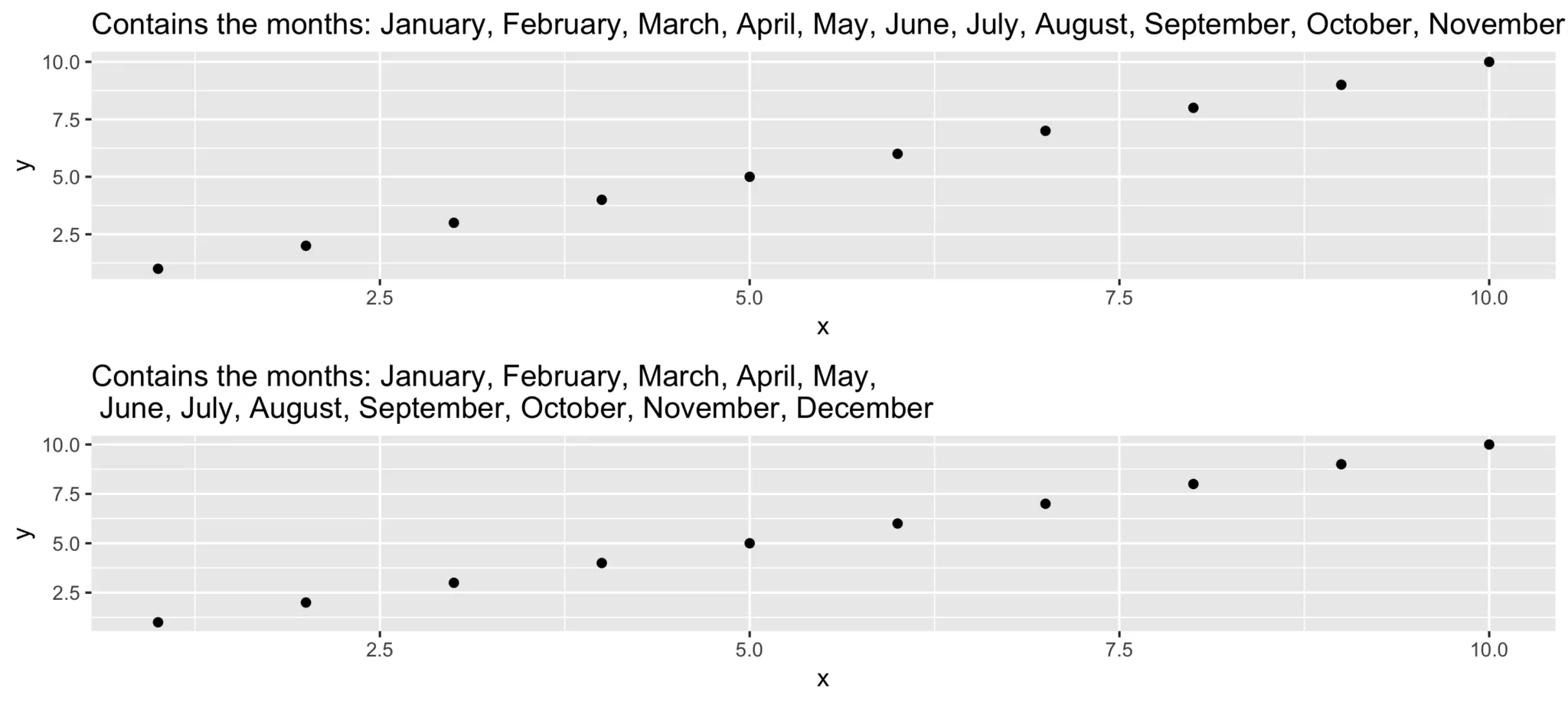
Code for plot example
p1 <- ggplot(data.frame(x = 1:10, y = 1:10),
  aes(x = x, y = y)) +
  geom_point() +
  ggtitle(long_title)

p2 <- ggplot(data.frame(x = 1:10, y = 1:10),
  aes(x = x, y = y)) +
  geom_point() +
  ggtitle(short_title)

multiplot(p1, p2)
6. get_files
This little helper does the same thing as the “Find in files” search within RStudio. It returns a vector with all files in a given folder that contain the search pattern. In your daily workflow, you would usually use the shortcut key SHIFT+CTRL+F. With get_files() you can use this functionality within your scripts.
7. get_network
This little helper aims to visualize the connections between R functions within a project as a flowchart. Herefore, the input is a directory path to the function or a list with the functions, and the outputs are an adjacency matrix and an igraph object. As an example, we use this folder with some toy functions:
net <- get_network(dir = "flowchart/R_network_functions/", simplify = FALSE)
g1 <- net(dollar sign)igraph
Input
There are five parameters to interact with the function:
- A path
dirwhich shall be searched. - A character vector
variationswith the function’s definition string -the default isc(" <- function", "<- function", "<-function"). - A
patterna string with the file suffix – the default is"\\.R(dollar sign)". - A boolean
simplifythat removes functions with no connections from the plot. - A named list
all_scripts, which is an alternative todir. This is mainly just used for testing purposes.
For normal usage, it should be enough to provide a path to the project folder.
Output
The given plot shows the connections of each function (arrows) and also the relative size of the function’s code (size of the points). As mentioned above, the output consists of an adjacency matrix and an igraph object. The matrix contains the number of calls for each function. The igraph object has the following properties:
- The names of the functions are used as label.
- The number of lines of each function (without comments and empty ones) are saved as the size.
- The folder‘s name of the first folder in the directory.
- A color corresponding to the folder.
With these properties, you can improve the network plot, for example, like this:
library(igraph)

# create plots ------------------------------------------------------------
l <- layout_with_fr(g1)
colrs <- rainbow(length(unique(V(g1)(dollar sign)color)))

plot(g1,
     edge.arrow.size = .1,
     edge.width = 5*E(g1)(dollar sign)weight/max(E(g1)(dollar sign)weight),
     vertex.shape = "none",
     vertex.label.color = colrs[V(g1)(dollar sign)color],
     vertex.label.color = "black",
     vertex.size = 20,
     vertex.color = colrs[V(g1)(dollar sign)color],
     edge.color = "steelblue1",
     layout = l)
legend(x = 0,
       unique(V(g1)(dollar sign)folder), pch = 21,
       pt.bg = colrs[unique(V(g1)(dollar sign)color)],
       pt.cex = 2, cex = .8, bty = "n", ncol = 1)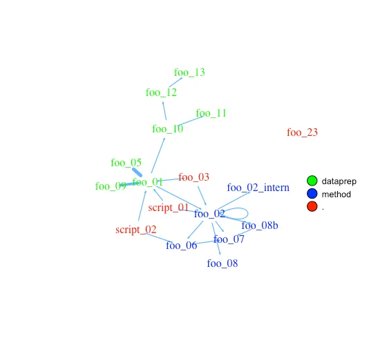
8. get_sequence
This little helper returns indices of recurring patterns. It works with numbers as well as with characters. All it needs is a vector with the data, a pattern to look for, and a minimum number of occurrences.
Let’s create some time series data with the following code.
library(data.table)

# random seed
set.seed(20181221)

# number of observations
n <- 100

# simulationg the data
ts_data <- data.table(DAY = 1:n, CHANGE = sample(c(-1, 0, 1), n, replace = TRUE))
ts_data[, VALUE := cumsum(CHANGE)]
This is nothing more than a random walk since we sample between going down (-1), going up (1), or staying at the same level (0). Our time series data looks like this:
Assume we want to know the date ranges when there was no change for at least four days in a row.
ts_data[, get_sequence(x = CHANGE, pattern = 0, minsize = 4)] min max
[1,] 45 48
[2,] 65 69
We can also answer the question if the pattern “down-up-down-up” is repeating anywhere:
ts_data[, get_sequence(x = CHANGE, pattern = c(-1,1), minsize = 2)] min max
[1,] 88 91
With these two inputs, we can update our plot a little bit by adding some geom_rect!
Code for the plot
rect <- data.table(
  rbind(ts_data[, get_sequence(x = CHANGE, pattern = c(0), minsize = 4)],
        ts_data[, get_sequence(x = CHANGE, pattern = c(-1,1), minsize = 2)]),
  GROUP = c("no change","no change","down-up"))

ggplot(ts_data, aes(x = DAY, y = VALUE)) +
  geom_line() +
  geom_rect(data = rect,
  inherit.aes = FALSE,
  aes(xmin = min - 1,
  xmax = max,
  ymin = -Inf,
  ymax = Inf,
  group = GROUP,
  fill = GROUP),
  color = "transparent",
  alpha = 0.5) +
  scale_fill_manual(values = statworx_palette(number = 2, basecolors = c(2,5))) +
  theme_minimal()
9. intersect2
This little helper returns the intersect of multiple vectors or lists. I found this function here, thought it is quite useful and adjusted it a bit.
intersect2(list(c(1:3), c(1:4)), list(c(1:2),c(1:3)), c(1:2))[1] 1 2
Internally, the problem of finding the intersection is solved recursively, if an element is a list and then stepwise with the next element.
10. multiplot
This little helper combines multiple ggplots into one plot. This is a function taken from the R cookbook.
An advantage over facets is, that you don’t need all data for all plots within one object. Also you can freely create each single plot – which can sometimes also be a disadvantage.
With the layout parameter you can arrange multiple plots with different sizes. Let’s say you have three plots and want to arrange them like this:
1    2    2
1    2    2
3    3    3
With multiplot it boils down to
multiplot(plotlist = list(p1, p2, p3),
          layout = matrix(c(1,2,2,1,2,2,3,3,3), nrow = 3, byrow = TRUE))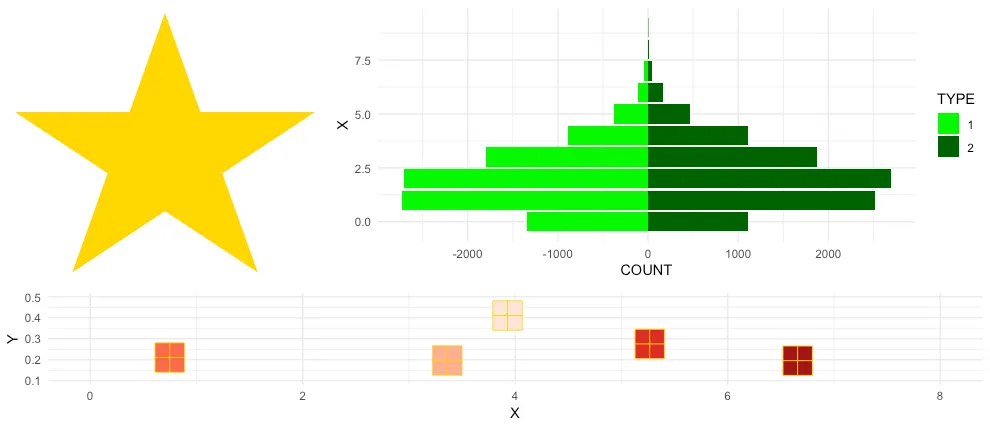
Code for plot example
# star coordinates
c1  =   cos((2*pi)/5)
c2  =   cos(pi/5)
s1  =   sin((2*pi)/5)
s2  =   sin((4*pi)/5)

data_star <- data.table(X = c(0, -s2, s1, -s1, s2),
                        Y = c(1, -c2, c1, c1, -c2))

p1 <- ggplot(data_star, aes(x = X, y = Y)) +
  geom_polygon(fill = "gold") +
  theme_void()

# tree
set.seed(24122018)
n <- 10000
lambda <- 2
data_tree <- data.table(X = c(rpois(n, lambda), rpois(n, 1.1*lambda)),
                        TYPE = rep(c("1", "2"), each = n))
data_tree <- data_tree[, list(COUNT = .N), by = c("TYPE", "X")]
data_tree[TYPE == "1", COUNT := -COUNT]

p2 <- ggplot(data_tree, aes(x = X, y = COUNT, fill = TYPE)) +
  geom_bar(stat = "identity") +
  scale_fill_manual(values = c("green", "darkgreen")) +
  coord_flip() +
  theme_minimal()

# gifts
data_gifts <- data.table(X = runif(5, min = 0, max = 10),
                         Y = runif(5, max = 0.5),
                         Z = sample(letters[1:5], 5, replace = FALSE))

p3 <- ggplot(data_gifts, aes(x = X, y = Y)) +
  geom_point(aes(color = Z), pch = 15, size = 10) +
  scale_color_brewer(palette = "Reds") +
  geom_point(pch = 12, size = 10, color = "gold") +
  xlim(0,8) +
  ylim(0.1,0.5) +
  theme_minimal() +
  theme(legend.position="none")
11. na_omitlist
This little helper removes missing values from a list.
y <- list(NA, c(1, NA), list(c(5:6, NA), NA, "A"))
There are two ways to remove the missing values, either only on the first level of the list or wihtin each sub level.
na_omitlist(y, recursive = FALSE)[[1]]
[1] 1 NA
[[2]]
[[2]][[1]]
[1] 5 6 NA
[[2]][[2]]
[1] NA
[[2]][[3]]
[1] "A"na_omitlist(y, recursive = TRUE)[[1]]
[1] 1
[[2]]
[[2]][[1]]
[1] 5 6
[[2]][[2]]
[1] "A"
12. %nin%
This little helper is just a convenience function. It is simply the same as the negated %in% operator, as you can see below. But in my opinion, it increases the readability of the code.
all.equal( c(1,2,3,4) %nin% c(1,2,5),
!c(1,2,3,4) %in% c(1,2,5))[1] TRUE
Also, this operator has made it into a few other packages as well – as you can read here.
13. object_size_in_env
This little helper shows a table with the size of each object in the given environment.
If you are in a situation where you have coded a lot and your environment is now quite messy, object_size_in_env helps you to find the big fish with respect to memory usage. Personally, I ran into this problem a few times when I looped over multiple executions of my models. At some point, the sessions became quite large in memory and I did not know why! With the help of object_size_in_env and some degubbing I could locate the object that caused this problem and adjusted my code accordingly.
First, let us create an environment with some variables.
# building an environment
this_env <- new.env()
assign("Var1", 3, envir = this_env)
assign("Var2", 1:1000, envir = this_env)
assign("Var3", rep("test", 1000), envir = this_env)
To get the size information of our objects, internally format(object.size()) is used. With the unit the output format can be changed (eg. "B", "MB" or "GB") .
# checking the size
object_size_in_env(env = this_env, unit = "B")
OBJECT SIZE UNIT
1: Var3 8104 B
2: Var2 4048 B
3: Var1 56 B
14. print_fs
This little helper returns the folder structure of a given path. With this, one can for example add a nice overview to the documentation of a project or within a git. For the sake of automation, this function could run and change parts wihtin a log or news file after a major change.
If we take a look at the same example we used for the get_network function, we get the following:
print_fs("~/flowchart/", depth = 4)1 flowchart
2 ¦--create_network.R
3 ¦--getnetwork.R
4 ¦--plots
5 ¦ ¦--example-network-helfRlein.png
6 ¦ °--improved-network.png
7 ¦--R_network_functions
8 ¦ ¦--dataprep
9 ¦ ¦ °--foo_01.R
10 ¦ ¦--method
11 ¦ ¦ °--foo_02.R
12 ¦ ¦--script_01.R
13 ¦ °--script_02.R
14 °--README.md
With depth we can adjust how deep we want to traverse through our folders.
15. read_files
This little helper reads in multiple files of the same type and combines them into a data.table. Which kind of file reading function should be used can be choosen by the FUN argument.
If you have a list of files, that all needs to be loaded in with the same function (e.g. read.csv), instead of using lapply and rbindlist now you can use this:
read_files(files, FUN = readRDS)
read_files(files, FUN = readLines)
read_files(files, FUN = read.csv, sep = ";")
Internally, it just uses lapply and rbindlist but you dont have to type it all the time. The read_files combines the single files by their column names and returns one data.table. Why data.table? Because I like it. But, let’s not go down the rabbit hole of data.table vs dplyr (to the rabbit hole …).
16. save_rds_archive
This little helper is a wrapper around base R saveRDS() and checks if the file you attempt to save already exists. If it does, the existing file is renamed / archived (with a time stamp), and the “updated” file will be saved under the specified name. This means that existing code which depends on the file name remaining constant (e.g., readRDS() calls in other scripts) will continue to work while an archived copy of the – otherwise overwritten – file will be kept.
17. sci_palette
This little helper returns a set of colors which we often use at statworx. So, if – like me – you cannot remeber each hex color code you need, this might help. Of course these are our colours, but you could rewrite it with your own palette. But the main benefactor is the plotting method – so you can see the color instead of only reading the hex code.
To see which hex code corresponds to which colour and for what purpose to use it
sci_palette(scheme = "new")Tech Blue Black White Light Grey Accent 1 Accent 2 Accent 3
"#0000FF" "#000000" "#FFFFFF" "#EBF0F2" "#283440" "#6C7D8C" "#B6BDCC"
Highlight 1 Highlight 2 Highlight 3
"#00C800" "#FFFF00" "#FE0D6C"
attr(,"class")
[1] "sci"
As mentioned above, there is a plot() method which gives the following picture.
plot(sci_palette(scheme = "new"))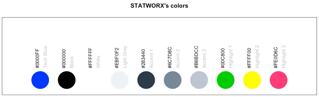
18. statusbar
This little helper prints a progress bar into the console for loops.
There are two nessecary parameters to feed this function:
runis either the iterator or its numbermax.runis either all possible iterators in the order they are processed or the maximum number of iterations.
So for example it could be run = 3 and max.run = 16 or run = "a" and max.run = letters[1:16].
Also there are two optional parameter:
percent.maxinfluences the width of the progress barinfois an additional character, which is printed at the end of the line. By default it isrun.
A little disadvantage of this function is, that it does not work with parallel processes. If you want to have a progress bar when using apply functions check out pbapply.
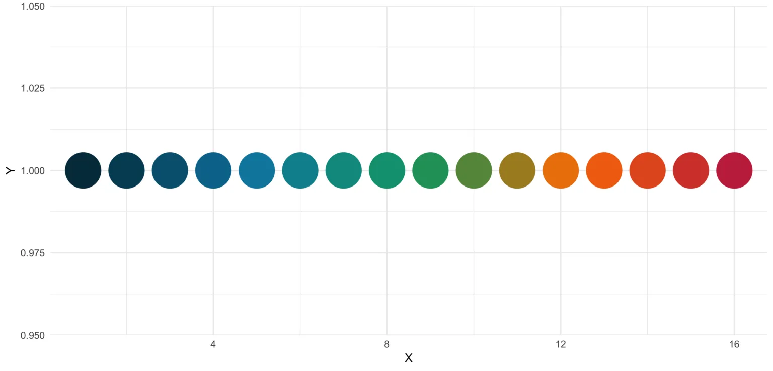
19. statworx_palette
This little helper is an addition to yesterday’s sci_palette(). We picked colors 1, 2, 3, 5 and 10 to create a flexible color palette. If you need 100 different colors – say no more!
In contrast to sci_palette() the return value is a character vector. For example if you want 16 colors:
statworx_palette(16, scheme = "old")[1] "#013848" "#004C63" "#00617E" "#00759A" "#0087AB" "#008F9C" "#00978E" "#009F7F"
[9] "#219E68" "#659448" "#A98B28" "#ED8208" "#F36F0F" "#E45A23" "#D54437" "#C62F4B"
If we now plot those colors, we get this nice rainbow like gradient.
library(ggplot2)

ggplot(plot_data, aes(x = X, y = Y)) +
  geom_point(pch = 16, size = 15, color = statworx_palette(16, scheme = "old")) +
  theme_minimal()
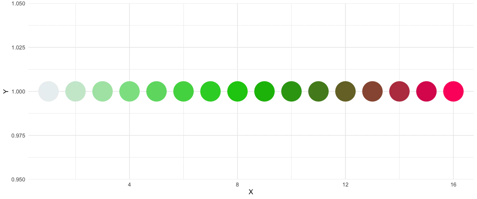
An additional feature is the reorder parameter, which samples the color’s order so that neighbours might be a bit more distinguishable. Also if you want to change the used colors, you can do so with basecolors.
ggplot(plot_data, aes(x = X, y = Y)) +
  geom_point(pch = 16, size = 15,
             color = statworx_palette(16, basecolors = c(4,8,10), scheme = "new")) +
  theme_minimal()
20. strsplit
This little helper adds functionality to the base R function strsplit – hence the same name! It is now possible to split before, after or between a given delimiter. In the case of between you need to specify two delimiters.
Here is a little example on how to use the new strsplit.
text <- c("This sentence should be split between should and be.")

strsplit(x = text, split = " ")
strsplit(x = text, split = c("should", " be"), type = "between")
strsplit(x = text, split = "be", type = "before")[[1]]
[1] "This" "sentence" "should" "be" "split" "between" "should" "and"
[9] "be."
[[1]]
[1] "This sentence should" " be split between should and be."
[[1]]
[1] "This sentence should " "be split " "between should and "
[4] "be."
21. to_na
This little helper is just a convenience function. Some times during your data preparation, you have a vector with infinite values like Inf or -Inf or even NaN values. Thos kind of value can (they do not have to!) mess up your evaluation and models. But most functions do have a tendency to handle missing values. So, this little helper removes such values and replaces them with NA.
A small exampe to give you the idea:
test <- list(a = c("a", "b", NA),
             b = c(NaN, 1,2, -Inf),
             c = c(TRUE, FALSE, NaN, Inf))

lapply(test, to_na)
(dollar sign)a
[1] "a" "b" NA
(dollar sign)b
[1] NA 1 2 NA
(dollar sign)c
[1] TRUE FALSE NA
A little advice along the way! Since there are different types of NA depending on the other values within a vector. You might want to check the format if you do to_na on groups or subsets.
test <- list(NA, c(NA, "a"), c(NA, 2.3), c(NA, 1L))
str(test)
List of 4
(dollar sign) : logi NA
(dollar sign) : chr [1:2] NA "a"
(dollar sign) : num [1:2] NA 2.3
(dollar sign) : int [1:2] NA 1
22. trim
This little helper removes leading and trailing whitespaces from a string. With R version 3.5.1 trimws was introduced, which does the exact same thing. This just shows, it was not a bad idea to write such a function. 😉
x <- c("  Hello world!", "  Hello world! ", "Hello world! ")
trim(x, lead = TRUE, trail = TRUE)[1] "Hello world!" "Hello world!" "Hello world!"
The lead and trail parameters indicates if only leading, trailing or both whitspaces should be removed.
Conclusion
I hope that the helfRlein package makes your work as easy as it is for us here at statworx. If you have any questions or input about the package, please send us an email to: blog@statworx.com


