How to Speed Up Gradient Boosting by a Factor of Two


Introduction
At statworx, we are not only helping customers find, develop, and implement a suitable data strategy but we also spend some time doing research to improve our own tool stack. This way, we can give back to the open-source community.
One special focus of my research lies in tree-based ensemble methods. These algorithms are bread and butter tools in predictive learning and you can find them as a standalone model or as an ingredient to an ensemble in almost every supervised learning Kaggle challenge. Renowned models are Random Forest by Leo Breiman, Extremely Randomized Trees (Extra-Trees) by Pierre Geurts, Damien Ernst & Louis Wehenkel, and Multiple Additive Regression Trees (MART; also known as Gradient Boosted Trees) by Jerome Friedman.
One thing I was particularly interested in, was how much randomization techniques have helped improve prediction performance in all of the algorithms named above. In Random Forest and Extra-Trees, it is quite obvious. Here, randomization is the reason why the ensembles offer an improvement over bagging; through the de-correlation of the base learners, the variance of the ensemble and therefore its prediction error decreases. In the end, you achieve de-correlation by “shaking up” the base trees, as it’s done in the two ensembles. However, MART also profits from randomization. In 2002, Friedman published another paper on boosting, showing that you can improve the prediction performance of boosted trees by training each tree on only a random subsample of your data. As a side-effect, your training time also decreases. Furthermore, in 2015, Rashmi and Gilad suggested adding a method known as a dropout to the boosting ensemble: a method found and used in neural nets.
The Idea behind Random Boost
Inspired by theoretical readings on randomization techniques in boosting, I developed a new algorithm, that I called Random Boost (RB). In its essence, Random Boost sequentially grows regression trees with random depth. More precisely, the algorithm is almost identical to and has the exact same input arguments as MART. The only difference is the parameter $d_{max}$. In MART $d_{max}$ determines the maximum depth of all trees in the ensemble. In Random Boost, the argument constitutes the upper bound of possible tree sizes. In each boosting iteration $i$, a random number $d_i$ between 1 and $d_{max}$ is drawn, which then defines the maximum depth of that tree $T_i(d_i)$.
In comparison to MART, this has two advantages:
First, RB is faster than MART on average, when being equipped with the same value for the tree size. When RB and MART are trained with a value for the maximum tree depth equal to $d_{max}$, then Random Boost will in many cases grow trees the size of $d$<$d_{max}$ by nature. If you assume that for MART, all trees will be grown to their full size $d_{max}$ (i.e. there is enough data left in each internal node so that tree growing doesn’t stop before the maximum size is reached), you can derive a formula showing the relative computation gain of RB over MART:
$t_{rel}(d_{max}) = frac{t_{mathrm{RB}}(d_{max})}{t_{mathrm{MART}}(d_{max})} approx frac{2}{d_{max}}left(1 - left(frac{1}{2}right)^{d_{max}} right).$
$t_{RB}(d_{max})$ e.g. is the training time of a RB boosting ensemble with the tree size parameter being equal to $d_{max}$.
To make it a bit more practical, the formula predicts that for $d_{max}=2, 3$ and $4$ takes $75%, 58%$ and $47%$ of the computation time of MART, respectively. These predictions, however, should be seen as RB’s best-case scenario, as MART is also not necessarily growing full trees. Still, the calculations suggest that efficiency gains can be expected (more on that later).
Second, there are also reasons to assume that randomizing over tree depths can have a beneficial effect on the prediction performance. As already mentioned, from a variance perspective, boosting suffers from overcapacity for various reasons. One of them is choosing too rich of a base learner in terms of depth. If, for example, one assumes that the dominant interaction in the data generating process is of order three, one would pick a tree with equivalent depth in MART in order to capture this interaction depth. However, this may be overkill, as fully grown trees with a depth equal to $3$ have eight leaves and therefore learn noise in the data, if there are only a few of such high order interactions. Perhaps, in this case, a tree with depth $3$but less than eight leaves would be optimal. This is not accounted for in MART, if one doesn’t want to add a pruning step to each boosting iteration at the expense of computational overhead. Random Boost may offer a more efficient remedy to this issue. With probability $1 / d_{max}$, a tree is grown, which is able to capture the high order effect at the cost of also learning noise. However, in all the other cases, Random Boost constructs smaller trees that do not show the over-capacity behavior and that can focus on interactions of smaller order. If over-capacity is an issue in MART due to different interactions in the data governed by a small number of high order interactions, Random Boost may perform better than MART. Furthermore, Random Boost also decorrelates trees through the extra source of randomness, which has a variance reducing the effect on the ensemble.
The concept of Random Boost constitutes a slight change to MART. I used the sklearn package as a basis for my code. As a result, the algorithm is developed based on sklearn.ensemle.GradientBoostingRegressor and sklearn.ensemle.GradientBoostingClassifier and is used in exactly the same way (i.e. argument names match exactly and CV can be carried out with sklearn.model_selection.GridSearchCV). The only difference is that the RandomBoosting*-object uses max_depth to randomly draw tree depths for each iteration. As an example, you can use it like this:
rb = RandomBoostingRegressor(learning_rate=0.1, max_depth=4, n_estimators=100)
rb = rb.fit(X_train, y_train)
rb.predict(X_test)
For the full code, check out my GitHub account.
Random Boost versus MART – A Simulation Study
In order to compare the two algorithms, I ran a simulation on 25 Datasets generated by a Random Target Function Generator that was introduced by Jerome Friedman in his famous Boosting paper he wrote in 2001 (you can find the details in his paper. Python code can be found here). Each dataset (containing 20,000 observations) was randomly split into a 25% test set and a 75% training set. RB and MART were tuned via 5-fold CV on the same tuning grid.
learning_rate = 0.1
max_depth = (2, 3, ..., 8)
n_estimators = (100, 105, 110, ..., 195)
For each dataset, I tuned both models to obtain the best parameter constellation. Then, I trained each model on every point of the tuning grid again and saved the test MAE as well as the total training time in seconds. Why did I train every model again and didn’t simply store the prediction accuracy of the tuned models along with the overall tuning time? Well, I wanted to be able to see how training time varies with the tree size parameter.
A Comparison of Prediction Accuracies
You can see the distribution of MAEs of the best models on all 25 datasets below.

Evidently, both algorithms perform similarly.
For a better comparison, I compute the relative difference between the predictive performance of RB and MART for each dataset $j$, i.e. $MAE_{rel,j}=frac{MAE_{RB,j}-MAE_{MART,j}}{MAE_{MART,j}}$. If $MAE_{rel,j}$>$0$, then RB had a larger mean absolute error than MART on dataset $j$, and vice versa.

In the majority of cases, RB did worse than MART in terms of prediction accuracy ($MAE_{rel}$>$0$). In the worst case, RB had a 1% higher MAE than MART. In the median, RB has a 0.19% higher MAE. I’ll leave itu p to you to decide whether that difference is practically significant.
A comparison of Training times
When we look at training time, we get a quite clear picture. In absolute terms, it took 433 seconds to train all parameter combinations of RB on average, as opposed to 803 seconds for MART.
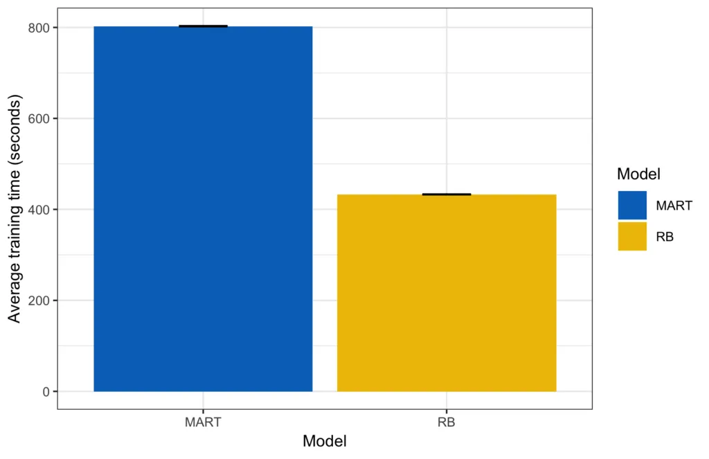
The small black lines on top of each bar are the error bars (2 times the means standard deviation; rather small in this case).
To give you a better feeling of how each model performed on each dataset, I also plotted the training times for each round.

If you now compute the training time ratio between MART and RB ($frac{t_{MART}}{t_{RB}}$), you see that RB is roughly 1.8 times faster than MART on average.
Another perspective on the case is to compute the relative training time $t_{rel,j}=frac{t_{RB,j}}{t_{MART,j}}$which is just 1 over the speedup. Note that this measure has to be interpreted a bit differently from the relative MAE measure above. If $t_{rel,j}=1$, then RB is as fast as MART, if $t_{rel,j}$>$1$, then it takes longer to train RB than MART, and if $t_{rel,j}$<$1$, then RB is faster than MART.
On average, RB only needs roughly 54% of MART’s tuning time in the median, and it is noticeably faster in all cases. I was also wondering how the relative training time varies with $d_{max}$ and how well the theoretically derived lower bound from above fits the actually measured relative training time. That’s why I computed the relative training time across all 25 datasets by tree size.
The theoretical figures are optimistic, but the relative performance gain of RB increases with tree size.
Results in a Nutshell and Next Steps
As part of my research on tree-based ensemble methods, I developed a new algorithm called Random Boost. Random Boost is based on Jerome Friedman’s MART, with the slight difference that it fits trees of random size. In total, this little change can reduce the problem of overfitting and noticeably speed up computation. Using a Random Target Function Generator suggested by Friedman, I found that, on average, RB is roughly twice as fast as MART with a comparable prediction accuracy in expectation.
Since running the whole simulation takes quite some time (finding the optimal parameters and retraining every model takes roughly one hour for each data set on my Mac), I couldn’t run hundreds or more simulations for this blog post. That’s the objective for future research on Random Boost. Furthermore, I want to benchmark the algorithm on real-world datasets.
In the meantime, feel free to look at my code and run the simulations yourself. Everything is on GitHub. Moreover, if you find something interesting and you want to share it with me, please feel free to shoot me an email.
References
- Breiman, Leo (2001). Random Forests. Machine Learning, 45, 5–32
- Chang, Tianqi, and Carlos Guestrin. 2016. XGBoost: A Scalable Tree Boosting System. Proceedings of the 22nd ACM SIGKDD International Conference on Knowledge Discovery and Data Mining, Pages 785-794
- Chapelle, Olivier, and Yi Chang. 2011. “Yahoo! learning to rank challenge overview”. In Proceedings of the Learning to Rank Challenge, 1–24.
- Friedman, J. H. (2001). Greedy function approximation: a gradient boosting machine. Annals of statistics, 1189-1232.
- Friedman, J. H. (2002). “Stochastic gradient boosting”. Computational Statistics & Data Analysis 38 (4): 367–378.
- Geurts, Pierre, Damien Ernst, and Louis Wehenkel (2006). “Extremely randomized trees”. Machine learning 63 (1): 3–42.
- Rashmi, K. V., and Ran Gilad-Bachrach (2015). Proceedings of the 18th International Conference on Artificial Intelligence and Statistics (AISTATS) 2015, San Diego, CA, USA. JMLR: W&CP volume 38.


