Introduction to Reinforcement Learning – When Machines Learn Like Humans


Most machine learning algorithms used in practice today belong to the class of supervised learning. In supervised learning, the machine learning model is presented ex post with an already known target variable $y$, which should be predicted as accurately as possible based on various influencing factors $X$ in the data through a function $f$. The function $f$ abstractly represents the respective machine learning model, which provides a mapping between the model's inputs and outputs.
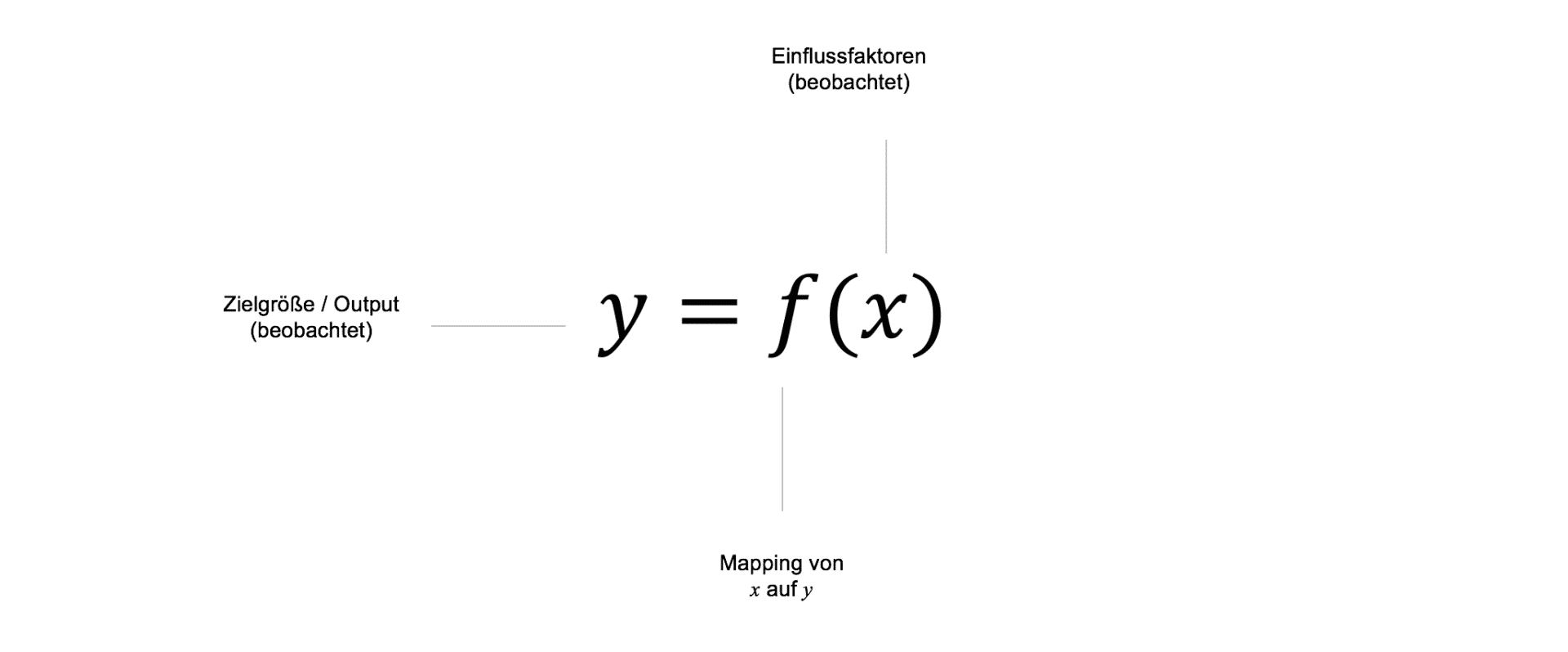
The learned target variables of simple ML models are therefore typically static and change only over historical time, which is already known ex post. Over time, new data points can be collected, which are then incorporated into the learned mapping $f$ between $X$ and $y$ in the form of "retraining".
Based on the predictions of a model, further actions—which are usually still human-controlled—are triggered. These actions often represent the actual decisions that lead to business-relevant impacts and implications. As a result, business decisions based on ML models are, in many cases, still not fully machine-controlled or only partially automated. Only in very few areas today are fully autonomous models applied, capable of making independent decisions and monitoring or adjusting their behavior in a model-based manner.
On the path toward self-learning, autonomous algorithms, which are necessary for artificial intelligence, models from supervised learning provide only a limited contribution.
On the path toward self-learning, autonomous algorithms, which are essential for artificial intelligence, models from supervised learning provide only a limited contribution. This is primarily due to the fact that the 1:1 relationship between inputs and outputs learned by machine learning models is insufficient for more complex scenarios or decision-making environments. For example, most machine learning models struggle to learn multiple target variables simultaneously or to capture a sequence of target variables and actions. Additionally, the relationship between influencing factors and target variables can immediately vary depending on the environment or based on previous predictions and decisions. This would imply a continuous retraining of models under changing conditions.
To enable machine learning models to be applied in environments where they can independently learn action-reaction events, learning methods are required that account for the dynamic nature of a changing environment. A well-known example of the successful application of such algorithms is Google’s AI AlphaGo, which defeated the world’s best human Go player. AlphaGo would have been impossible to develop using classical supervised learning methods since, due to the infinite number of moves and scenarios, no model would have been capable of mapping the complexity of action-reaction relationships as a simple input-output function. Instead, methods are needed that can autonomously respond to new environmental conditions, anticipate possible future actions, and incorporate them into current decision-making. The class of learning methods on which systems like AlphaGo are based is called reinforcement learning.
What is Reinforcement Learning?
Reinforcement Learning (RL), alongside Supervised Learning and Unsupervised Learning, represents the third major category of machine learning methods. RL is a method inspired by the natural learning behavior of humans. Human learning, especially in early stages, often occurs through simple exploration of the environment. In a learning problem, our actions are defined within a certain action space. Through trial and error, we observe and evaluate the effects of different actions on our environment. In response to our actions, we receive feedback from our environment, abstractly represented in the form of rewards or punishments. However, the concept of reward or punishment should rarely be understood monetarily. In many cases, rewards come in the form of social acceptance, praise from others, personal well-being, or a sense of achievement. Often, there is also a temporal delay between an action and its reward. Humans typically aim not just to maximize immediate rewards, but rather to maximize their total expected reward over time through their actions.
An example: When learning to play the guitar, our action space consists of plucking the strings and pressing down on the fretboard. Through initially random exploration of these actions, we receive feedback from the environment in the form of sounds produced by the guitar. We are rewarded when the notes sound clear and punished when our neighbors bang on the ceiling with a broom. Our goal is to maximize the total expected reward in the form of correctly played notes and chords over our relevant time horizon. This does not mean that we stop learning as soon as we can play a single chord correctly—instead, it manifests through continuous training and the constant pursuit of new rewards and successes that await us over time. Naturally, the duration of exploration of possible actions and environmental rewards can be improved by introducing an external trainer. This example is, of course, highly simplified, but it effectively conveys the core principle of Reinforcement Learning.
Formally, Reinforcement Learning consists of five key components: (1) the agent, (2) the environment, (3) the state, (4) the action, and (5) the reward. The general process can be described as follows: The agent performs an action ($a_t$) from the available action space ($A$) in a given environment at a specific state ($s_t$), which leads to a response from the environment in the form of a reward ($r_t$).

The environment's reaction to the agent's action then influences the agent's choice of action in the next state $s_{t+1}$. Over thousands, hundreds of thousands, or even millions of iterations, the agent can approximate the relationship between its actions and the expected future reward in each state, allowing it to behave optimally.
The agent constantly faces a dilemma between exploiting its previously acquired experience and exploring new strategies to increase its reward. This is known as the "exploration-exploitation dilemma." The approximation of rewards can be model-free, meaning it occurs purely through exploration of the environment, or it can be achieved using machine learning models that attempt to approximate the value of an action. The latter approach is particularly useful when the state and/or action space is high-dimensional.
Q-Learning
To train Reinforcement Learning systems, a commonly used method is Q-Learning. The name Q-Learning comes from the so-called Q-function $Q(s,a)$, which describes the expected reward $Q$ of an action $a$ in state $s$. The Q-values are stored in the Q-matrix $Q$, whose dimensionality is defined by the number of possible states and actions. During training, the agent attempts to approximate the Q-values of the Q-matrix through exploration, so that these values can later be used as a decision rule. The reward matrix $R$ contains, corresponding to $Q$, the respective rewards the agent receives for each state-action pair.
The approximation of Q-values works in its simplest form as follows: The agent starts in a randomly initialized state$s_t$. The agent then randomly selects an action$a_t$ from $A$, observes the corresponding reward$r_t$, and the next state$s_{t+1}$. The update rule of the Q-matrix is defined as follows:
$$Q(s_t,a_t)=(1-\alpha)Q(s_t, a_t)+\alpha(r_t+\gamma \max Q(s_{t+1},a))$$
The Q-value in state $s_t$ for executing action $a_t$ is a function of the already learned Q-value (first part of the equation) and the reward in the current state, plus the discounted maximum Q-value of all possible actions $a$ in the next state $s_{t+1}$.
The parameter $\alpha$, found in the first part of the equation, is called the learning rate and controls the extent to which newly observed information influences the agent’s decision to take a specific action.
The parameter $\gamma$ is known as the discount factor, which manages the trade-off between short-term and future rewards in the agent’s decision-making process. Smaller $\gamma$ values make the agent favor immediate rewards, while larger $\gamma$ values encourage the agent to prioritize long-term rewards in decision-making.
In model-based Q-Learning environments, exploration of the environment does not occur purely randomly. Instead, Q-values in the Q-matrix are approximated using machine learning models, typically neural networks and deep learning models. During training, model-based RL systems often include a random action component, where the agent executes an action with a probability $p \lt \epsilon$. This approach is called $\epsilon$-greedy and is designed to prevent the agent from always selecting the same actions during exploration.
After the learning phase, the agent selects the action with the highest Q-value in each state, $\max Q(s_t, a)$. This allows the agent to move from state to state, always choosing the action that maximizes the approximated reward.
Q-Learning is particularly useful when the number of possible states and actions remains manageable. Otherwise, due to combinatorial complexity, solving the problem with pure exploration mechanisms becomes difficult. For this reason, in high-dimensional state and action spaces, the approximation of Q-values is often performed using model-based approaches.
Another challenge in applying Q-Learning arises when rewards are temporally distant from the agent’s current state and action space. If no rewards exist in nearby states, the agent requires a long exploration phase before it can propagate rewards from distant future states back to its current decision-making process.
Minimal Example for Q-Learning
The new autonomous vacuum robot "Dusty3000" from the company DUSTWORX is designed to navigate unknown apartments fully autonomously. The device uses a Reinforcement Learning approach to determine which rooms in an apartment accumulate dust and lint. A virtual test apartment, where the robot is calibrated, has the following layout:
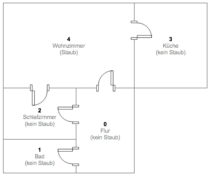
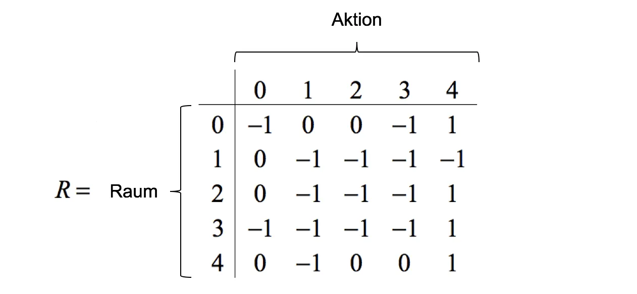
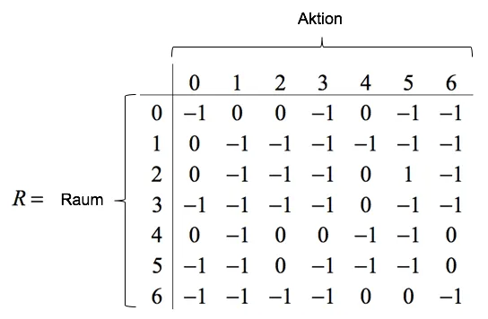
The virtual test apartment consists of five rooms, but in this test scenario, dust is only present in the living room. If the robot finds its way to the dust, it receives a reward of $r = 1$; otherwise, no reward is given($r = 0$). Rooms that the robot cannot reach from its current position are assigned $r = -1$ in the reward matrix. In matrix notation, the rewards and the possible actions per room are represented as follows:
Let’s assume the vacuum robot starts its exploration randomly in the hallway (room 0). From its current state ($s = 0$), the robot has three possible actions: 1, 2, or 4. Actions 0 and 3 are not possible because these rooms cannot be reached directly from the hallway. The agent receives no reward if it chooses action $a = 1$, moving from the hallway to room 1 (bathroom). The same applies to action $a = 2$ (moving into the bedroom). However, if the robot chooses action $a = 4$ and moves into the living room, it finds the dust and receives a reward of $r = 1$. For an external observer, the optimal action seems obvious, but our robot does not know its environment and randomly selects from the available actions.
The robot begins its random exploration of the apartment. The learning rate is set to $\alpha = 1$, and the discount factor is set to $\gamma = 0.95$. Starting in the hallway, it selects action $a = 2$ randomly from the available actions. As a result, the robot moves into the bedroom. In the simplified case where $\alpha = 1.0$, the Q-value for moving from the hallway to the bedroom is defined as follows:
$$Q(0,2)=(1-\alpha)Q(0,2)+\alpha(r_t+\gamma \max Q(s_{t+1},a))$$$$=(1-1)*0+1*(0+0.95\max[Q(2,0),Q(2,4)])$$$$=0+1*(0+0.95 \max[0, 1])=0.95$$
Here, the importance of the discount factor becomes evident: If the discount factor were 0, the possibility of moving from the bedroom to the living room would not be considered when initially moving from the hallway to the bedroom. This would result in a Q-value of $Q(0,2) = 0$. However, since the discount factor in our example is greater than 0, the potential future reward is also incorporated into $Q(0,2)$.
Upon arriving in the bedroom, the robot again has two possible actions: It can either move back to the hallway ($a = 0$) or continue moving into the living room ($a = 4$). By chance, the robot chooses the living room, resulting in the following Q-value:
$$Q(2,4)=(1-\alpha)+\alpha(r_t+\gamma \max Q(s_{t+1},a)) $$$$=(1-1)*0+1*(1+0.95\max[Q(4,0),Q(4,3)]) $$$$ =0+1*(1+0.95\max[0,0])=1$$
The entire process from exploration to receiving a reward is called an episode. Since the robot has now reached its goal, the episode ends. During this iteration, the agent was able to calculate two Q-values, which are stored in the Q-matrix—essentially serving as the robot’s memory.
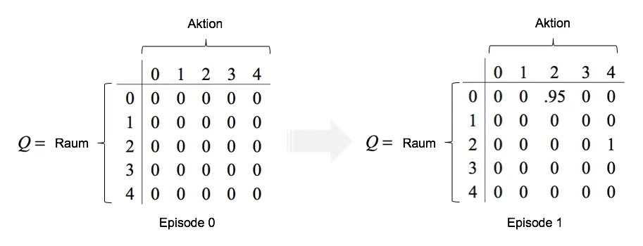
As training progresses, the values in the Q-matrix are updated step by step by the algorithm. The robot selects the action with the highest Q-value in each room. The exploration of the environment ends when the agent receives a reward.
Implementation in Python
To illustrate the example above, the following Python code implements the algorithm. First, a function is created that executes the described algorithm based on the reward matrix $R$, the learning rate $\alpha$, the discount factor $\gamma$, and the number of episodes.
# Imports
import numpy as np

# Funktion
def q_learning(R, gamma, alpha, episodes):

    """ Funktion für Q Learning """

    # Anzahl der Zeilen und Spalten der R-Matrix
    n, p = R.shape

    # Erstellung der Q Matrix (0-Werte)
    Q = np.zeros(shape=[n, p])

    # Loop Episoden
    for i in range(episodes):

        # Zufälliger Startpunkt des Roboters
        state = np.random.randint(0, n, 1)

        # Iteration
        for j in range(100):

            # Mögliche Rewards im aktuellen Status
            rewards = R[state]

            # Mögliche Bewegungen des Roboters im aktuellen Status
            possible_moves = np.where(rewards[0] > -1)[0]

            # Zufällige Bewegung des Roboters
            next_state = np.random.choice(possible_moves, 1)

            # Update der Q values berechnen
            Q[state, next_state] = (1 - alpha) * Q[state, next_state] + alpha * (
                R[state, next_state] + gamma * np.max(Q[next_state, :]))

            # Abbrechen der Episode wenn Ziel erreicht
            if R[state, next_state] == 1:
                break

    # Q-Matrix zurückgeben
    return Q
First, the number of states $n$ and the number of actions $p$ are determined. These values are derived from the reward matrix $R$. Next, an initially empty matrix $Q$ is created to store the Q-values during the learning process. Inside the loop over the specified number of episodes $episodes$, the agent starts at a randomly selected position. The described algorithm is then executed in $j=100$ iterations: From the set of possible actions $possible_moves$ for the current state $state$, a random action is selected and stored in the variable $next_state$. Then, the Q-values are updated according to the formula described above. Here, both the current Q-value at $Q[state, next_state]$ and the reward of the current state $R[state, next_state]$ are processed. After updating the Q-values, it is checked whether the agent has received a reward. If so, the inner loop terminates, and the simulation proceeds to the next episode. After all episodes are completed, the final Q-matrix is returned.
A practical application of the above function is shown in the code box below. First, the reward matrix is defined in analogy to the example described earlier, and then passed to the q_learning function along with the other parameters. The learning rate is set to $\alpha=0.8$, and the discount factor is set to $\gamma=0.95$. A total of $n=1000$ episodes are simulated.
# Anzahl der Räume
rooms = 5

# Belohnungs-Matrix
R = np.zeros(shape=[rooms, rooms])
R[0, :] = [-1,  0,  0, -1,  1]
R[1, :] = [ 0, -1, -1, -1, -1]
R[2, :] = [ 0, -1, -1, -1,  1]
R[3, :] = [-1, -1, -1, -1,  1]
R[4, :] = [ 0, -1,  0,  0,  1]

# Q-Learning
Q = q_learning(R=R, gamma=0.95, alpha=0.8, episodes=1000)

# Finale Q Matrix normalisieren und anzeigen
np.round(Q / np.max(Q), 4)
array([[ 0.    ,  0.9025,  0.95  ,  0.    ,  1.    ],
       [ 0.95  ,  0.    ,  0.    ,  0.    ,  0.    ],
       [ 0.95  ,  0.    ,  0.    ,  0.    ,  1.    ],
       [ 0.    ,  0.    ,  0.    ,  0.    ,  1.    ],
       [ 0.95  ,  0.    ,  0.95  ,  0.95  ,  1.    ]])
At the final Q-matrix, the learned actions of the robot can now be read. This is done by identifying the maximum Q-value per state (row). Example: If the robot is in the hallway (row 1 of the matrix), the maximum Q-value is found in the last column. This corresponds to a movement into the living room. If the agent is in the bathroom (row 2), it first moves into the hallway (row 1). From there, the maximum Q-value determines a movement into the living room.
A more complex example
Our Dusty3000 has already proven itself in the simple simulation environment. Now, we want to determine how the robot can navigate more complex apartments. For this purpose, the apartment has been expanded by two additional rooms, and the dust has been moved from the living room to the children's room:
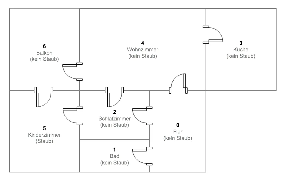
The children's room is significantly more difficult to reach compared to the previous example and can only be accessed through various paths. As a result, the robot will have a harder time correctly estimating the Q-values. The reward matrix is adjusted accordingly as follows:
Analogous to the previous example, the learning rate is set to $\alpha=0.8$ and the discount factor to $\gamma=0.95$. A total of $n=1000$ episodes are simulated.
# Anzahl der Räume
rooms = 7

# Belohnungs-Matrix
R = np.zeros(shape=[rooms, rooms])
R[0, :] = [-1,  0,  0, -1,  0, -1, -1]
R[1, :] = [ 0, -1, -1, -1, -1, -1, -1]
R[2, :] = [ 0, -1, -1, -1,  0,  1, -1]
R[3, :] = [-1, -1, -1, -1,  0, -1, -1]
R[4, :] = [ 0, -1,  0,  0, -1, -1,  0]
R[5, :] = [-1, -1,  0, -1, -1, -1,  0]
R[6, :] = [-1, -1, -1, -1,  0,  0, -1]

# Q-Learning!
Q = q_learning(R=R, gamma=0.95, alpha=0.8, episodes=1000)

# Normalize
np.round(Q / np.max(Q), 4)
array([[ 0.    ,  0.8571,  0.9499,  0.    ,  0.9023,  0.    ,  0.    ],
       [ 0.9023,  0.    ,  0.    ,  0.    ,  0.    ,  0.    ,  0.    ],
       [ 0.9023,  0.    ,  0.    ,  0.    ,  0.9023,  1.    ,  0.    ],
       [ 0.    ,  0.    ,  0.    ,  0.    ,  0.9023,  0.    ,  0.    ],
       [ 0.9023,  0.    ,  0.9497,  0.857 ,  0.    ,  0.    ,  0.857 ],
       [ 0.    ,  0.    ,  0.9499,  0.    ,  0.    ,  0.    ,  0.8571],
       [ 0.    ,  0.    ,  0.    ,  0.    ,  0.9023,  0.9023,  0.    ]])
The resulting Q-matrix is more complex than in the simpler previous example. Example: Starting from the hallway (row 1), the agent moves into room 2 (bedroom) and from there into the children's room, where the reward awaits. Starting from the kitchen (row 4), the robot moves into the living room (row 5), then into the bedroom (row 3), and finally into the children's room.
Conclusion and outlook
With Reinforcement Learning and Q-Learning, it is possible to develop algorithms and systems that autonomously learn and execute actions in both deterministic and stochastic environments without knowing them explicitly. The agent always attempts to maximize the reward generated by the environment based on its actions. The discount factor can be used to control whether the agent should focus on short-term or long-term rewards. The application areas for such agents are diverse and exciting: Some time ago, Google published a paper in which an agent was trained using model-based Reinforcement Learning to play various Atari computer games. In the next stage of development, the previously developed RL system DQN (Deep Q-Network) was applied to the significantly more complex strategy game classic StarCraft. Unlike the example shown here, the derivation of the optimal action was not solved using a matrix-based overview but through Deep Learning models that approximate the Q-values in $s_{t+1}$ based on the pixels on the screen. We will explore this application in the second part of the Reinforcement Learning series and demonstrate how neural networks and Deep Learning can be used as Q-approximators. This opens up significantly more complex and realistic applications, as the number of states can be arbitrarily high.
References
- Sutton, Richard S.; Barto, Andrew G. (1998). Reinforcement Learning: An Introduction. MIT Press.
- Goodfellow, Ian; Bengio Yoshua; Courville, Cohan (2016). Deep Learning. MIT Press.


