How do neural networks learn?


For outsiders, neural networks often carry a mystical aura. While the fundamental building blocks of neural networks—known as neurons—have been understood for many decades, training these networks remains a challenge for practitioners even today. This is especially true in the field of deep learning, where highly deep or otherwise complex network architectures are valued. The way a network learns from available data plays a crucial role in the success of its training.
This article explores the two fundamental components of neural network learning: (1) Gradient Descent, an iterative optimization method used to minimize functions, and (2) Backpropagation, a technique for determining the magnitude and direction of parameter adjustments in a neural network. The combination of these two methods enables us to develop and train a wide variety of model types and architectures using available data.
Formal Structure of a Neuron
A neuron $j$ computes its output $o_j$ as a weighted sum of its input signals $x$, which is then transformed by an activation function, denoted as $g(x)$. The choice of activation function for $g()$ significantly influences the functional output of the neuron. The following diagram provides a schematic representation of a single neuron.
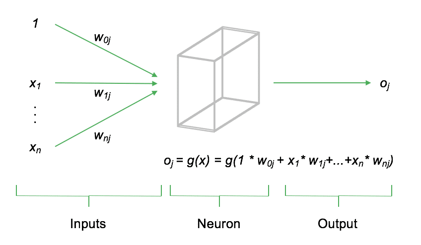
In addition to the inputs $x_1, \dots, x_n$, each neuron includes a so-called bias. The bias regulates the neuron's baseline activation level and is an essential component of the neuron. Both the input values and the bias are combined as a weighted sum before being passed into the neuron. This weighted sum is then non-linearly transformed by the neuron's activation function.
Today, the Rectified Linear Unit (ReLU) is one of the most commonly used activation functions. It is defined as: $g(x) = \max(0, x)$. Other activation functions include the sigmoid function, defined as: $g(x) = \frac{1}{1+e^{-x}}$ as well as the hyperbolic tangent (tanh) function: $g(x) = 1 - \frac{2}{e^{2x} + 1}$.
The following Python code provides an example of how to compute the output of a neuron.
# Imports
import numpy as np

# ReLU Aktivierungsfunktion
def relu(x):
    """ ReLU Aktivierungsfunktion """
    return(np.maximum(0, x))

# Funktion für ein einzelnes Neuron
def neuron(w, x):
    """ Neuron """
    # Gewichtete Summe von w und x
    ws = np.sum(np.multiply(w, x))
    # Aktivierungsfunktion (ReLU)
    out = relu(ws)
    # Wert zurückgeben
    return(out)

# Gewichtungen und Inputs
w = [0.1, 1.2, 0.5]
x = [1, 10, 10]

# Berechnung Output (ergibt 18.0)
p = neuron(w, x)
array([18.0])
Through the application of the ReLU activation function, the output of the neuron in the above example is 181818. Naturally, a neural network does not consist of just one neuron but rather a large number of neurons, which are interconnected through weight parameters in layers. By combining many neurons, the network is capable of learning highly complex functions.
Gradient Descent
Simply put, neural networks learn by iteratively comparing model predictions with the actual observed data and adjusting the weight parameters in the network so that, in each iteration, the error between the model's prediction and the actual data is reduced. To quantify the model error, a so-called cost function is computed. The cost function typically has two input arguments: (1) the model's output, $o$, and (2) the actual observed data, $y$. A common cost function frequently used in neural networks is the Mean Squared Error (MSE):
$E = \frac{1}{n} \sum (y_i - o_i)^2$
The MSE first computes the squared difference between $y$ and $o$ for each data point and then takes the average. A high MSE reflects poor model fit to the given data. The goal of model training is to minimize the cost function by adjusting the model parameters (weights). How does the neural network determine which weights need to be adjusted and, more importantly, in which direction?
The cost function depends on all parameters in the neural network. Even a minimal change in a single weight has a direct impact on all subsequent neurons, the network's output, and thus also on the cost function. In mathematics, the magnitude and direction of change in the cost function due to a change in a single parameter can be determined by computing the partial derivative of the cost function with respect to the corresponding weight parameter: $\frac{\partial E}{\partial w_{ij}}$. Since the cost function $E$ hierarchically depends on the different weight parameters in the network, the chain rule for derivatives can be applied to derive the following equation for updating the weights in the network:
$w_{ij,t} = w_{ij,t-1} - \eta \frac{\partial E}{\partial w_{ij}}$
The adjustment of the weight parameters from one iteration to the next in the direction of cost function minimization depends solely on the value of the respective weight from the previous iteration, the partial derivative of $E$ with respect to $w_{ij}$, and a learning rate $\eta$. The learning rate determines the step size in the direction of error minimization. The approach outlined above, where the cost function is iteratively minimized based on gradients, is referred to as Gradient Descent. The following diagram illustrates the influence of the learning rate on the minimization of the cost function (adapted from Yann LeCun).
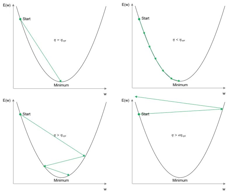
Ideally, the learning rate would be set in such a way that the minimum of the cost function is reached in just one iteration (top left). Since the theoretically correct value is not known in practice, the learning rate must be defined by the user. In the case of a small learning rate, one can be relatively certain that a (at least local) minimum of the cost function will be reached. However, in this scenario, the number of iterations required to reach the minimum increases significantly (top right). If the learning rate is chosen larger than the theoretical optimum, the path toward the minimum becomes increasingly unstable. While the number of iterations decreases, it cannot be guaranteed that a local or global optimum will actually be reached. Especially in regions where the slope or surface of the error curve becomes very flat, an excessively large step size may cause the minimum to be missed (bottom left). If the learning rate is significantly too high, this leads to a destabilization of the minimization process, and no meaningful solution for adjusting the weights is found (bottom right). In modern optimization schemes, adaptive learning rates are also used, which adjust the learning rate throughout training. For example, a higher learning rate can be chosen at the beginning, which is then gradually reduced over time to more reliably converge to the (local) optimum.
# Imports
import numpy as np

# ReLU Aktivierungsfunktion
def relu(x):
    """ ReLU Aktivierungsfunktion """
    return(np.maximum(0, x))


# Ableitung der Aktivierungsfunktion
def relu_deriv(x):
    """ Ableitung ReLU """
    return(1)


# Kostenfunktion
def cost(y, p):
    """ MSE Kostenfunktion """
    mse = np.mean(pow(y-p, 2))
    return(mse)


# Ableitung der Kostenfunktion
def cost_deriv(y, p):
    """ Ableitung MSE """
    return(y-p)


# Funktion für ein einzelnes Neuron
def neuron(w, x):
    """ Neuron """
    # Gewichtete Summe von w und x
    ws = np.sum(np.multiply(w, x))
    # Aktivierungsfunktion (ReLU)
    out = relu(ws)
    # Wert zurückgeben
    return(out)


# Initiales Gewicht
w = [5.5]

# Input
x = [10]

# Target
y = [100]

# Lernrate
eta = 0.01

# Anzahl Iterationen
n_iter = 100

# Neuron trainieren
for i in range(n_iter):
    # Ausgabe des Neurons berechnen
    p = neuron(w, x)
    # Ableitungen berechnen
    delta_cost = cost_deriv(p, y)
    delta_act = relu_deriv(x)
    # Gewichtung aktualisieren
    w = w - eta * delta_act * delta_cost

# Ergebnis des Trainings
print(w)
array([9.99988047])
Through the iterative training of the model, the input weights have been adjusted in such a way that the difference between the model prediction and the actual observed value is close to 0. This can be easily verified:
$o_j = g(x) = g(w \cdot x) = \max(0, 9.9998 \times 10) = \max(0, 99.998) = 99.998$
Thus, the result is almost 100. The mean squared error (MSE) is $3.9999e-06$, which is also close to 0. The following figure provides a final visualization of the MSE during the training process.
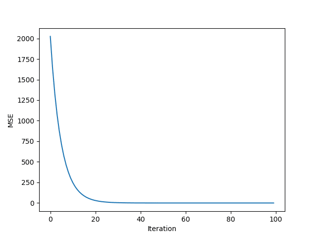
One can clearly see the monotonically decreasing mean squared error. After 30 iterations, the error is practically zero.
Backpropagation
The previously described method of steepest gradient descent is still used today to minimize the cost function of neural networks. However, computing the necessary gradients in more complex network architectures is significantly more challenging than in the simple example of a single neuron shown above. The reason for this is that the gradients of individual neurons depend on each other, meaning that there is a chain of dependencies between neurons in the network. To address this issue, the so-called Backpropagation Algorithm is used, which enables the recursive calculation of gradients in each iteration.
Originally developed in the 1970s, the Backpropagation Algorithm only gained widespread recognition in 1986 through the groundbreaking paper by Rumelhart, Hinton, and Williams (1986), where it was used for training neural networks for the first time. The complete formal derivation of the Backpropagation Algorithm is too complex to be presented in detail here. Instead, the following provides a formal outline of its fundamental workflow.
In matrix notation, the vector of outputs $o_l$ for all neurons in a layer $l$ is defined as
$o_l = g(w_l o_{l-1} + b_l)$
where $w_l$ represents the weight matrix between the neurons of layers $l$ and $l-1$, and $o_{l-1}$ denotes the output of the previous layer. The term $b_l$ represents the bias values of layer $l$. The function $g$ is the activation function of the layer. The term inside the parentheses is also referred to as the weighted input $z$, so it follows that $o_l = g(z)$ with $z = w_l o_{l-1} + b_l$. Furthermore, we assume that the network consists of a total of $L$ layers. The output of the network is therefore $o_L$. The cost function $E$ of the neural network must be defined in such a way that it can be expressed as a function of the output $o_L$ and the observed data $y$.
The change in the cost function with respect to the weighted input of a neuron $j$ in layer $l$ is defined as $\delta_j = \frac{\partial E}{\partial z_j}$. The larger this value, the stronger the dependence of the cost function on the weighted input of this neuron. The change in the cost function with respect to the outputs of the output layer $L$ is defined as
$\delta_L = \frac{\partial E}{\partial o_L} g'(z_L)$
The exact form of $\delta_L$ depends on the choice of cost function $E$. The mean squared error (MSE) used here can be derived with respect to $o_L$ as follows:
$\frac{\partial E}{\partial o_L} = (y - o_L)$
Thus, the gradient vector for the output layer can be written as
$\delta_L = (y - o_L) g'(z_L)$
For the preceding layers $l = 1, \dots, L-1$, the gradient vector is given by
$\delta_l = (w_{l+1})^T \delta_{l+1} g'(z_l)$
As shown, the gradients in layer $l$ are a function of the gradients and weights of the following layer $l+1$. Therefore, it is essential to begin the gradient calculations in the final layer of the network and propagate them iteratively backward through the previous layers (Backpropagation). By combining $\delta_L$ and $\delta_l$, the gradients for all layers in the neural network can be computed. Once the gradients for all layers in the network are known, the weights in the network can be updated using Gradient Descent. This update is applied in the opposite direction of the computed gradients, thereby reducing the cost function. For the following programming example, which illustrates the Backpropagation Algorithm, we extend our neural network from the previous example by adding an additional neuron. The network now consists of two layers—the hidden layer and the output layer. The hidden layer continues to use the ReLU activation function, while the output layer applies a linear activation function, meaning it simply forwards the weighted sum of the neuron.
# Neuron
def neuron(w, x, activation):
    """ Neuron """
    # Gewichtete Summe von w und x
    ws = np.sum(np.multiply(w, x))
    # Aktivierungsfunktion (ReLU)
    if activation == 'relu':
        out = relu(ws)
    elif activation == 'linear':
        out = ws
    # Wert zurückgeben
    return(out)


# Initiale Gewichte
w = [1, 1]

# Input
x = [10]

# Target
y = [100]

# Lernrate
eta = 0.001

# Anzahl Iterationen
n_iter = 100

# Container für Gradienten
delta = [0, 0]

# Container für MSE
mse = []

# Anzahl Layer
layers = 2

# Neuron trainieren
for i in range(100):
    # Hidden layer
    hidden = neuron(w[0], x, activation='relu')
    # Output layer
    p = neuron(w[1], x=hidden, activation='linear')
    # Ableitungen berechnen
    d_cost = cost_deriv(p, y)
    d_act = relu_deriv(x)
    # Backpropagation
    for l in reversed(range(layers)):
        # Output Layer
        if l == 1:
            # Gradienten und Update
            delta[l] = d_act * d_cost
            w[l] = w[l] - eta * delta[l]
        # Hidden Layer
        else:
            # Gradienten und Update
            delta[l] = w[l+1] * delta[l+1] * d_act
            w[l] = w[l] - eta * delta[l]
    # Append MSE
    mse.append(cost(y, p))

# Ergebnis des Trainings
print(w)
[array([3.87498172]), array([2.58052067])]
Unlike the previous example, the loop has now become slightly more complex by adding an additional loop. This additional loop implements backpropagation within the network. Using reversed(range(layers)), the loop iterates backward over the number of layers, starting at the output layer. The gradients are then computed according to the formula presented above, followed by updating the weights using gradient descent. Multiplying the computed weights yields
$3.87498172 \times 10 \times 2.58052067 = 99.99470$
which is once again very close to the target value of $y = 100$. Through the application of backpropagation and gradient descent, the (albeit very minimalistic) neural network has successfully learned the target value.
Summary and Outlook
Today, neural networks learn using gradient descent (or modern variations of it) and backpropagation. The development of more efficient learning methods that are faster, more precise, and more stable than existing forms of backpropagation and gradient descent remains a key research area in this field. This is particularly important for deep learning models, where very deep architectures need to be optimized, making the choice of learning method crucial for both the training speed and the accuracy of the model. The fundamental mechanisms of learning algorithms for neural networks have remained largely unchanged over time. However, driven by extensive research in this domain, it is possible that a new learning algorithm will emerge in the future—one that is just as revolutionary and successful as the backpropagation algorithm.


