Data Science in Python - The Core of it All - Part 2


In the previous part of this statworx series, we dealt with various data structures. Among them were those that are available in Python directly 'out of the box' as well as NumPy's ndarrays. With the native containers (e.g., tuples or lists), we found that only lists meet our requirements in the context of working with data—modifiable and indexable. However, these were relatively inflexible and slow once we attempted to use them for computationally intensive mathematical operations. For one, we had to apply operations on individual elements via loops, and applications from linear algebra, like matrix multiplication, were not possible. Hence, we turned our attention to NumPy's ndarrays. As NumPy forms the core of the scientific Python environment, we will focus more closely on arrays in this part. We will delve deeper into their structure and examine where the improved performance comes from. Finally, we will discuss how to save and reload your analysis or results.
Attributes and Methods
N-Dimensions
Like all constructs in Python, ndarrays are objects with methods and attributes. Besides efficiency, the most interesting attribute or feature for us is multidimensionality. As we saw in the last part, it is easy to create a two-dimensional array without nesting objects into each other, as would be the case with lists. Instead, we can simply specify the size of the respective object, with any dimensionality being chosen. Typically, this is indicated through the ndim argument. NumPy additionally offers us the ability to restructure arbitrarily large arrays exceptionally simply. The restructuring of an ndarray's dimensionality is done through the reshape() method. It is passed a tuple or list with the corresponding size. To obtain a restructured array, the number of elements must be compatible with the specified size.
# 2D-List
list_2d = [[1,2], [3,4]]

# 2D-Array
array_2d = np.array([1,2,3,4]).reshape((2,2))

# 10D-Array
array_10d = np.array(range(10), ndmin=10)
To obtain structural information about an array, such as dimensionality, we can call the attributes ndim, shape, or size. For example, ndim provides insight into the number of dimensions, while size tells us how many elements are in the respective array. The attribute shape combines this information and indicates how the respective entries are distributed across the dimensions.
# Creation of a 3x3x3 array with numbers 0 through 26
Arr = np.arange(3*3*3).reshape(3,3,3)

# Number of dimensions
Arr.ndim # =3

# Number of elements, 27
Arr.size # =27

# Detailed breakdown of these two pieces of information
Arr.shape # = (3,3,3) Three elements per dimension
Indexing
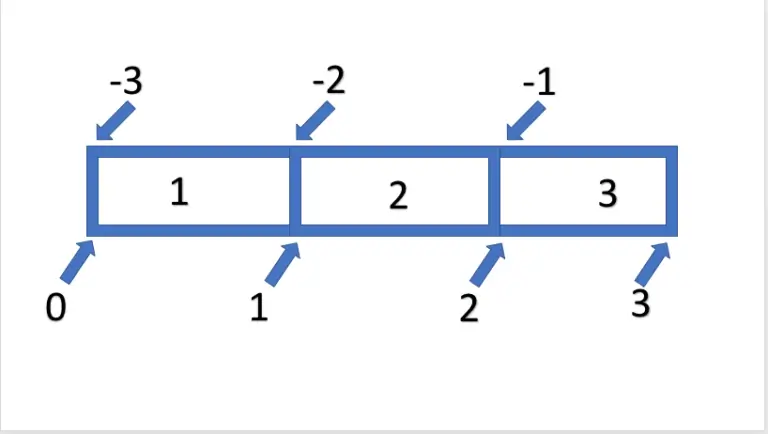
Now that we can determine how our ndarray is structured, the question arises: how can we select individual elements or sections of an array? This indexing, or slicing, is done similarly to lists. Using the [] notation, we can also retrieve a single index or entire sequences using the :- syntax for arrays. Indexing by index is relatively simple. For example, we obtain the first value of the array with Arr[0], and by preceding with a -, we obtain the last value of the array with Arr[-1]. However, if we want to retrieve a sequence of data, we can use the :- syntax. This follows the schema [ Start : End : Step ], with all arguments being optional. It should be noted that only the data exclusive of the specified end is output. Thus, Arr[0:2] gives us only the first two entries. The topic is illustrated in the following graphic.
If we want to select the entire array using this logic, we can also omit the start and/or end, which will be automatically supplemented. So, we could select from the first to the second element with Arr[:2] or from the second to the last element with Arr[1:].
Next, we want to address the previously omitted argument, step. This allows us to define the step size between the elements between start and end. If we want only every second element of the entire array, we can omit the start and end and define only a step size of 2 – Arr[::2]. As with reversed indexing, a reversed step size through negative values is also possible. Consequently, a step size of -1 results in the array being output in reverse order.
arrarr = np.array([1,1,2,2,3,3])
arr = np.array([1,2,3])
arrarr[::2] == arr
rra = np.array([3,2,1])
arr[::-1] == rra & rra[::-1] ==arr
True
If we now want to transfer this to an array that is not in a one-dimensional space but in a multidimensional space, we can simply consider each additional dimension as another axis. Consequently, we can relatively easily transfer slicing from a one-dimensional array to higher dimensions. For this, we only need to split each dimension individually and separate the individual commands with commas. To select an entire matrix of size 3x3 using this syntax, we need to select the entire first and second axes. Analogous to before, we would use [:] twice. This would be formulated in parentheses as [:,:]. This schema can be extended to any number of axes. Here are a few more examples:
arr = np.arange(8).reshape((2,2,2))
# the whole array
arr[:,:,:]
# the first element
arr[0,0,0]
# the last element
arr[-1,-1,-1]
Calculating with Arrays
UFuncs
As mentioned repeatedly in this and the last post, the great strength of NumPy lies in the fact that calculating with ndarray is extremely performant. The reason for this initially lies in the arrays, which are an efficient storage and enable higher-dimensional spaces to be mathematically represented. However, the great advantage of NumPy lies primarily in the functions provided to us. These functions make it possible to no longer iterate over individual elements via loops but to pass the entire object and also return only one. These functions are called 'UFuncs' and are characterized by being constructed and compiled to work on an entire array. All functions accessible to us through NumPy have these properties, including the np.sqrt function we used in the last part. Additionally, specially defined mathematical operators for arrays, such as +, -, *, ..., are also included. As these are ultimately only methods of an object (e.g., a.__add__(b) is the same as a + b), the operators for NumPy objects were implemented as Ufunc methods to ensure efficient computation. The corresponding functions could also be directly addressed:
Dynamic Dimensions via Broadcasting
Another advantage of arrays is that a dynamic adjustment of dimensions takes place through broadcasting as soon as a mathematical operation is executed. If we want to multiply a 3x1 vector and a 3x3 matrix element-wise, this would not be trivial to solve in algebra. NumPy 'stretches' the vector into another 3x3 matrix and then performs the multiplication.
The adjustment takes place according to three rules:
- Rule 1: If two arrays differ in the number of dimensions, the smaller array is adjusted with additional dimensions on the left side, e.g., (3,2) -> (1,3,2)
- Rule 2: If the arrays do not match in any dimension, the array with a unary dimension is stretched, as was the case in the example above (3x1) -> 3x3
- Rule 3: If neither Rule 1 nor Rule 2 applies, an error is generated.
# Rule 1
arr_1 = np.arange(6).reshape((3,2))
arr_2 = np.arange(6).reshape((1,3,2))
arr_2*arr_1 # ndim = 1,3,2

# Rule 2
arr_1 = np.arange(6).reshape((3,2))
arr_2 = np.arange(2).reshape((2))
arr_2*arr_1 # ndim = 3,2

# Rule 3
arr_1 = np.arange(6).reshape((3,2))
arr_2 = np.arange(6).reshape((3,2,1))
arr_2*arr_1 # Error, as it would need to fill on the right and not the left
ValueErrorTraceback (most recent call last)
<ipython-input-4-d4f0238d53fd> in <module>()
12 arr_1 = np.arange(6).reshape((3,2))
13 arr_2 = np.arange(6).reshape((3,2,1))
---> 14 arr_2*arr_1 # EError, as it would need to fill on the right and not the left
ValueError: operands could not be broadcast together with shapes (3,2,1) (3,2)At this point, it should be noted that broadcasting only applies to element-wise operations. If we use matrix multiplication, we must ensure that our dimensions match. If we want to multiply a 3x1 matrix with an array of size 3, as an example, the small matrix is not extended to the left as in Rule 2, but an error is directly generated.
arr_1 = np.arange(3).reshape((3,1))
arr_2 = np.arange(3).reshape((3))

# Error
arr_1@arr_2
ValueErrorTraceback (most recent call last)
<ipython-input-5-8f2e35257d22> in <module>()
3
4 # Error
----> 5 arr_1@arr_2
ValueError: shapes (3,1) and (3,) not aligned: 1 (dim 1) != 3 (dim 0)
Aggregation as an example of broadcasting should be more familiar and understandable than this dynamic adjustment.
In addition to the direct functions for sum or average, these can also be mapped via operators. Thus, the sum of an array can be obtained not only via np.sum(x, axis=None) but also via np.add.reduce(x, axis=None). This form of operator broadcasting allows us to apply the respective operation cumulatively to obtain rolling values. By specifying the axis, we can determine along which axis the operation should be executed. In the case of np.sum or np.mean, None is the default. This means that all axes are included, and a scalar is created. If we want to reduce the array by only one axis, we can specify the respective axis index:
# Reduce all axes
np.add.reduce(arr_1, axis=None)

# Reduce the third axes
np.add.reduce(arr, axis=2)

# Cumulative sum
np.add.accumulate(arr_1)

# Cumulative product
np.multiply.accumulate(arr_1)
Saving and Loading Data
Finally, we want to be able to save our results and load them again next time. In NumPy, we generally have two options. Number 1 is the use of text-based formats such as .csv through savetxt and loadtxt. Let's take a look at the main features of these functions, with all arguments listed for completeness, but only referring to the most important ones.
Saving data is done, as the name suggests, through the function:
np.savetxt(fname, X, fmt='%.18e', delimiter=' ', newline='n', header='', footer='', comments='# ', encoding=None)
Through this command, we can save an object X in a file fname. It is essentially irrelevant in which format we want to save it, as the object is saved in plain text. Thus, it does not matter whether we append txt or csv as a suffix; the names are simply conventions. Which values are used for separation are specified through the keywords delimiter and newline, which, in the case of a csv, are ',' for separating individual values/columns and n for a new row. Optionally, we can specify whether we want to write additional (string) information at the beginning or the end of the file using header and footer. By specifying fmt – which stands for format – we can influence whether and how the individual values should be formatted, i.e., whether, how, and how many places before and after the comma should be displayed. This way, we can make the numbers more readable or reduce the need for storage space on the hard drive by lowering precision. A simple example would be fmt = %.2, which rounds all numbers to the second decimal place (2.234 -> 2.23).
Loading previously saved data is done through the loadtxt function, which has many arguments that match the functions for saving objects.
np.loadtxt(fname, dtype=<class 'float'>, comments='#', delimiter=None, converters=None, skiprows=0, usecols=None, unpack=False, ndmin=0, encoding='bytes')
The arguments fname and delimiter have the same functionality and default values as when saving data. Through skiprows, it can be specified whether and how many rows should be skipped, and through usecols, a list of indices determines which columns should be read.
# Create an example
x = np.arange(100).reshape(10,10)

# Save it as CSV
np.savetxt('example.txt',x)

# Reload
x = np.loadtxt(fname='example.txt')

# Skip the first five rows
x = np.loadtxt(fname='example.txt', skiprows=5)

# Load only the first and last column
x = np.loadtxt(fname='example.txt', usecols= (0,-1))
The second option for saving data is binary .npy files. This results in compressed data, which requires less storage space but is no longer directly readable, like txt or csv files. Furthermore, the options for loading and saving are comparatively limited.
np.save(file, arr, allow_pickle=True, fix_imports=True)np.load(file, mmap_mode=None, allow_pickle=True, fix_imports=True, encoding='ASCII')
For us, only file and arr are interesting. As the name likely suggests, we can use the file argument to indicate in which file our array arr should be saved. Similarly, when loading, we can also determine the file to be loaded via load.
# Compress and save
np.save('example.npy', x )

# Load the compressed file
x = np.load('example.npy')
Preview
Now that we have familiarized ourselves with the mathematical core of the data science environment, we can engage in giving our data more content structure in the next part. For this, we will explore the next major library – namely Pandas. We will become acquainted with the two main objects – Series and DataFrame – of the library, which allow us to use existing datasets and directly modify and manipulate them.


