Data Science in Python - Preview and tools

Part 0 – Preview and Tools
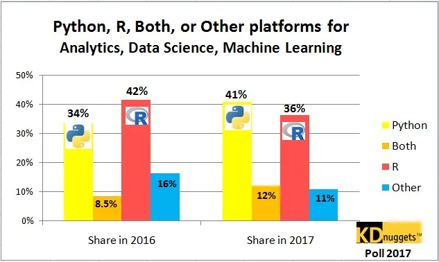
When it comes to data preparation, data formatting, and statistical analysis—or simply Data Science—R was (and still is here in Germany) the language of choice. Globally, however, Python has gained significantly in popularity and is now even dominant in this field (see the study by KDnuggets). Therefore, this series is intended to provide an initial insight into “Why Python?” and how the language operates in areas of “data science.” Accordingly, we will first address the question “Why Python?” as well as describe some useful tools.
This is followed by a look at data structures in Python using Pandas, as well as the mathematical ecosystem with NumPy and SciPy. To visualize our observations or mathematical transformations, we will take a brief look at Matplotlib. Most interesting, however, is the validation of given hypotheses or assumptions we have about our data, which we will perform using Statsmodels or SciKit-Learn (SKLearn). The problem up to this point is that almost all these Python modules and extensions are very basic frameworks. In other words, if you know what you want and how to use these tools, they are extremely powerful. However, this requires intensive engagement with their objects and functions. For this reason, various wrappers have been developed around these libraries to simplify our lives.
When it comes to statistical visualization, Seaborn now does the heavy lifting for us, and for those who prefer interactive graphics, Bokeh and Altair provide assistance. Even for machine learning (ML), there are numerous wrappers, such as MlXtend for the classical field or Keras in the area of deep learning.
Why Python
Accordingly, the journey begins with the justification of itself – Why Python? In contrast to R, Python is a general-purpose language. As a result, Python is not only more flexible in handling non-numerical objects, but also offers, through its object-oriented programming approach (OOP), the ability to freely manipulate or create any object. This becomes especially apparent when a dataset is either very “messy” or the information it contains is insufficient. In Python, numerous libraries are available to clean data in unconventional ways or to directly search or scrape the World Wide Web for information. While this can also be done in R, it usually requires significantly more effort. However, as soon as you move even further away from the actual data (e.g., setting up an API), R has to admit defeat entirely.
In this context, I would like to emphasize once again that when it comes to numerical objects and handling (relatively clean) data, Python will always lag slightly behind R. On the one hand, because R was written precisely for this purpose, and on the other hand, because the latest research results are first implemented in R. This is exactly where you can decide which language offers you more. If you always want to be up to date, apply the latest methods and algorithms, and focus on the essentials, then R is probably the better choice. But if you would rather build data pipelines, find a solution for every problem, and stay close to your data at all times, then Python is likely the better option.
Tools
ToolsBefore we now turn to Pandas and the core area of Data Science, I would like to introduce a multifunctional tool that has become virtually indispensable in my daily routine: Jupyter. It is an extension of the IPython console and allows you to write your code in different cells, execute it, and thus effectively divide long scripts.
#Definition of a function in a cell
def sayhello(to ):
    'Print hello to somboday'
    print(f'Hello {to}')

def returnhello(to):
    'Return a string which says Hello to somboday'
    return f'Hello {to}'
# Call this function in another cell
# Writes the message
sayhello('Statworx-Blog')# Introspection of the docstring
returnhello?Hello Statworx-Blog# returns an object which is formatted by the notebook
returnhello('Statworx-Blog') 'Hello Statworx-Blog'
What makes it special is both the interactive element—for example, you can quickly and easily get feedback at any time on what an object looks like—and IDE elements such as introspection using ?. Jupyter particularly shines through its beautiful visualization. As can be seen in the third cell (returnhello('Statworx-Blog')), the last object in a cell is always visualized. In this case, it may have just been a string, which of course we could simply output using print. However, we will see later on that this visualization is incredibly useful, especially with data. Moreover, the blocks can also be interpreted differently. For example, they can be left in their raw state without being compiled or used as Markdown to document the code alongside (or to write this post here).
Since Jupyter Notebooks are ultimately based on the IPython shell, we can of course also use all its features and magics. This allows for automatic completions. You get access to the docstrings of individual functions and classes, as well as line and cell magics in IPython. Individual blocks can therefore be used for more than just Python code. For example, code can be quickly and easily checked for its speed using %timeit, the system shell can be accessed directly using %%bash, or its output can be captured directly using ! at the beginning of the line. Furthermore, Ruby code could also be executed using %%ruby, JavaScript with %%js, or even switch between Python2 and Python3 using %%python2 & %%python3 in the respective cell.
%timeit returnhello('Statworx-Blog')170 ns ± 3.77 ns per loop (mean ± std. dev. of 7 runs, 10000000 loops each)%%bash
lsBlog_Python.html
Blog_Python.ipynb
Blog_Python.md
One note that must not be left out here is that Jupyter is not exclusive to Python but can also be used with R or Julia. While the respective kernels are not included “out of the box,” if you want or need to use another language, in my opinion, the minimal effort is worth it.
For those who don’t like the whole thing and prefer a good old IDE for Python, there are a variety of options available. Various multi-language IDEs with a Python plug-in (Visual Studio, Eclipse, etc.) or those tailored specifically to Python. The latter include PyCharm and Spyder.
PyCharm was developed by JetBrains and is available in two versions, the Community Edition (CE) and the Pro version. While the CE is an open-source project with “only” an intelligent editor, graphical debugger, VCS support, and introspection, the Pro version, available for a fee, includes support for web development. While this ensures the maintenance of the IDE, I personally miss the optimization for data science-specific applications (IPython console). Spyder, however, as a scientific open-source project, offers everything one could wish for. An editor (not quite as intelligent as the JetBrains version) for scripts, an explorer for variables and files, and an IPython console.
The last tool that is needed and must not be missing is an editor. Above all, it should be fast so that any file can at least be opened in raw format. This is necessary because a quick glance, for example into CSV files, often gives you a sense of the encoding: which character separates rows and which separates columns. On the other hand, it also allows you to quickly and easily open other scripts without having to wait for the IDE to load.
Preview
Now that we have an arsenal of tools to dive into data munging, in the next part of this series we can jump straight into Pandas, its DataFrames, and the mathematical ecosystem.


