Using Reinforcement Learning to play Super Mario Bros on NES using TensorFlow


Reinforcement learning is currently one of the hottest topics in machine learning. For a recent conference we attended (the awesome Data Festival in Munich), we’ve developed a reinforcement learning model that learns to play Super Mario Bros on NES so that visitors, that come to our booth, can compete against the agent in terms of level completion time.

The promotion was a great success and people enjoyed the “human vs. machine” competition. There was only one contestant who was able to beat the AI by taking a secret shortcut, that the AI wasn’t aware of. Also, developing the model in Python was a lot of fun. So, I decided to write a blog post about it that covers some of the fundamental concepts of reinforcement learning as well as the actual implementation of our Super Mario agent in TensorFlow (beware, I’ve used TensorFlow 1.13.1, TensorFlow 2.0 was not released at the time of writing this article).
Recap: reinforcement learning
Most machine learning models have an explicit connection between inputs and outputs that does not change during training time. Therefore, it can be difficult to model or predict systems, where the inputs or targets themselves depend on previous predictions. However, often,the world around the model updates itself with every prediction made. What sounds quite abstract is actually a very common situation in the real world: autonomous driving, machine control, process automation etc. – in many situations, decisions that are made by models have an impact on their surroundings and consequently on the next actions to be taken. Classical supervised learning approaches can only be used to a limited extend in such kinds of situations. To solve the latter, machine learning models are needed that are able to cope with time-dependent variation of inputs and outputs that are interdependent. This is where reinforcement learning comes into play.
In reinforcement learning, the model (called agent) interacts with its environment by choosing from a set of possible actions (action space) in each state of the environment that cause either positive or negative rewards from the environment. Think of rewards as an abstract concept of signalizing that the action taken was good or bad. Thereby, the reward issued by the environment can be immediate or delayed into the future. By learning from the combination of environment states, actions and corresponsing rewards (so called transitions), the agent tries to reach an optimal set of decision rules (the policy) that maximize the total reward gathered by the agent in each state.
Q-learning and Deep Q-learning
In reinforcement learning we often use a learning concept called Q-learning. Q-learning is based on so called Q-values, that help the agent determining the optimal action, given the current state of the environment. Q-values are “discounted” future rewards, that our agent collects during training by taking actions and moving through the different states of the environment. Q-values themselves are tried to be approximated during training, either by simple exploration of the environment or by using a function approximator, such as a deep neural network (as in our case here). Mostly, we select in each state the action that has the highest Q-value, i.e. the highest discounuted future reward, givent the current state of the environment.
When using a neural network as a Q-function approximator we learn by computing the difference between the predicted Q-values and the “true” Q-values, i.e. the representation of the optimal decision in the current state. Based on the computed loss, we update the network’s parameters using gradient descent, just like in any other neural network model. By doing this often, our network converges to a state, where it can approximate the Q-values of the next state, given the current state of the environment. If the approximation is good enough, we simple select the action that has the highest Q-value. By doing so, the agent is able to decide in each situation, which action generates the best outcome in terms of reward collection.
In most deep reinforcement learning models there are actually two deep neural networks involved: the online- and the target-network. This is done because during training, the loss function of a single neural network is computed against steadily changing targets (Q-values), that are based on the networks weights themselves. This adds increased difficulty to the optimization problem or might result in no convergence at all. The target network is basically a copy of the online network with frozen weights that are not directly trained. Instead the target network’s weights are synchronized with the online network after a certain amount of training steps. Enforcing “stable outputs” of the target network that do not change after each training step makes sure that the computed target Q-values that are needed for computing the loss do not change steadily which supports convergence of the optimization problem.
Deep Double Q-learning
Another possible issue with Q-learning is, that due to the selection of the maximum Q-value for determining the best action, the model sometimes produces extraordinary high Q-values during training. Basically, this is not always a problem but might turn into one, if there is a strong concentration at certain actions that in return lead to the negletion of less favorable but “worth-to-try” actions. If the latter are neglected all the time, the model might run into a locally optimal solution or even worse selects the same actions all the time. One way to deal with this problem is to introduce an updated version of Q-learning called double Q-learning.
In double Q-learning the actions in each state are not simply chosen by selecting the action with maximum Q-value of the target network. Instead, the selection process is split into three distinct steps: (1) first, the target network computes the target Q-values of the state after taking the action. Then, (2) the online network computes the Q-values of the state after taking the action and selects the best action by finding the maximum Q-value. Finally, (3) the target Q-Values are calculated using the target Q-values of the target network, but at the selected action indices of the online network. This assures, that there cannot occur an overestimation of Q-values because the Q-values are not updated based on themselves.
Gym environments
In order to build a reinforcement learning aplication, we need two things: (1) an environment that the agent can interact with and learn from (2) the agent, that observes the state(s) of the environment and chooses appropriate actions using Q-values, that (ideally) result in high rewards for the agent. An environment is typically provided as a so called gym, a class that contains the neecessary code to emulate the states and rewards of the environment as a function of the agent’s actions as well further information, e.g. about the possible action space. Here is an example of a simple environment class in Python:
class Environment:
    """ A simple environment skeleton """
    def __init__(self):
          # Initializes the environment
        pass

    def step(self, action):
          # Changes the environment based on agents action
        return next_state, reward, done, info

    def reset(self):
        # Resets the environment to its initial state
        pass

    def render(self):
          # Show the state of the environment on screen
        pass
The environment has three major class functions: (1) step() executes the environment code as function of the action selected by the agent and returns the next state of the environment, the reward with respect to action, a done flag indicating if the environment has reached its terminal state as well as a dictionary of additional information about the environment and its state, (2) reset() resets the environment in it’s original state and (3) render() print the current state on the screen (for example showing the current frame of the Super Mario Bros game).
For Python, a go-to place for finding gyms is OpenAI. It contains lots of diffenrent games and problems well suited for solving using reinforcement learning. Furthermore, there is an Open AI project called Gym Retro that contains hundrets of Sega and SNES games, ready to be tackled by reinforcement learning algorithms.
Agent
The agent comsumes the current state of the environment and selects an appropriate action based on the selection policy. The policy maps the state of the environment to the action to be taken by the agent. Finding the right policy is a key question in reinforcement learning and often involves the usage of deep neural networks. The following agent simply observes the state of the environment and returns action = 1 if state is larger than 0 and action = 0 otherwise.
class Agent:
    """ A simple agent """
    def __init__(self):
        pass

    def action(self, state):
        if state > 0:
            return 1
        else:
            return 0
This is of course a very simplistic policy. In practical reinforcement learning applications the state of the environment can be very complex and high-dimensional. One example are video games. The state of the environment is determined by the pixels on screen and the previous actions of the player. Our agent needs to find a policy that maps the screen pixels into actions that generate rewards from the environment.
Environment wrappers
Gym environments contain most of the functionalities needed to use them in a reinforcement learning scenario. However, there are certain features that do not come prebuilt into the gym, such as image downscaling, frame skipping and stacking, reward clipping and so on. Luckily, there exist so called gym wrappers that provide such kinds of utility functions. An example that can be used for many video games such as Atari or NES can be found here. For video game gyms it is very common to use wrapper functions in order to achieve a good performance of the agent. The example below shows a simple reward clipping wrapper.
import gym

class ClipRewardEnv(gym.RewardWrapper):
        """ Example wrapper for reward clipping """
    def __init__(self, env):
        gym.RewardWrapper.__init__(self, env)

    def reward(self, reward):
        # Clip reward to {1, 0, -1} by its sign
        return np.sign(reward)
From the example shown above you can see, that it is possible to change the default behavior of the environment by “overwriting” its core functions. Here, rewards of the environment are clipped to [-1, 0, 1] using np.sign() based on the sign of the reward.
The Super Mario Bros NES environment
For our Super Mario Bros reinforcement learning experiment, I’ve used gym-super-mario-bros. The API ist straightforward and very similar to the Open AI gym API. The following code shows a random agent playing Super Mario. This causes Mario to wiggle around on the screen and – of course – does not lead to a susscessful completion of the game.
from nes_py.wrappers import BinarySpaceToDiscreteSpaceEnv
import gym_super_mario_bros
from gym_super_mario_bros.actions import SIMPLE_MOVEMENT


# Make gym environment
env = gym_super_mario_bros.make('SuperMarioBros-v0')
env = BinarySpaceToDiscreteSpaceEnv(env, SIMPLE_MOVEMENT)

# Play random
done = True
for step in range(5000):
    if done:
        state = env.reset()
    state, reward, done, info = env.step(env.action_space.sample())
    env.render()

# Close device
env.close()
The agent interacts with the environment by choosing random actions from the action space of the environment. The action space of a video game is actually quite large since you can press multiple buttons at the same time. Here, the action space is reduced to SIMPLE_MOVEMENT, which covers basic game actions such as run in all directions, jump, duck and so on. BinarySpaceToDiscreteSpaceEnv transforms the binary action space (dummy indicator variables for all buttons and directions) into a single integer. So for example the integer action 12 corresponds to pressing right and A (running).
Using a deep learning model as an agent
When playing Super Mario Bros on NES, humans see the game screen – more precisely – they see consecutive frames of pixels, displayed at a high speed on the screen. Our human brains are capable of transforming the raw sensorial input from our eyes into electrical signals that are processed by our brain that trigger corresponding actions (pressing buttons on the controller) that (hopefully) lead Mario to the finishing line.
When training the agent, the gym renders each game frame as a matrix of pixels, according to the respective action taken by the agent. Basically, those pixels can be used as an input to any machine learning model. However, in reinforcement learning we often use convolutional neural networks (CNNs) that excel at image recognition problems compared to other ML models. I won’t go into technical detail about CNNs here, there’s a plethora of great intro articles to CNNs like this one.
Instead of using only the current game screen as an input to the model, it is common to use multiple stacked frames as an input to the CNN. By doing so, the model can process changes and “movements” on the screen between consecutive frames, which would not be possible when using only a single game frame. Here, the input tensor of our model is of size [84, 84, 4]. This corresponds to a stack of 4 grayscale frames, each frame of size 84×84 pixels. This corresponds to the default tensor size for 2-dimensional convolution.
The architecture of the deep learning model consists of three convolutional layers, followed by a flatten and one fully connected layer with 512 neurons as well as an output layer, consisting of actions = 6 nerons, which corresponds to the action space of the game (in this case RIGHT_ONLY, i.e. actions to move Mario to the right – enlarging the action space usually causes an increase in problem complexity and training time).
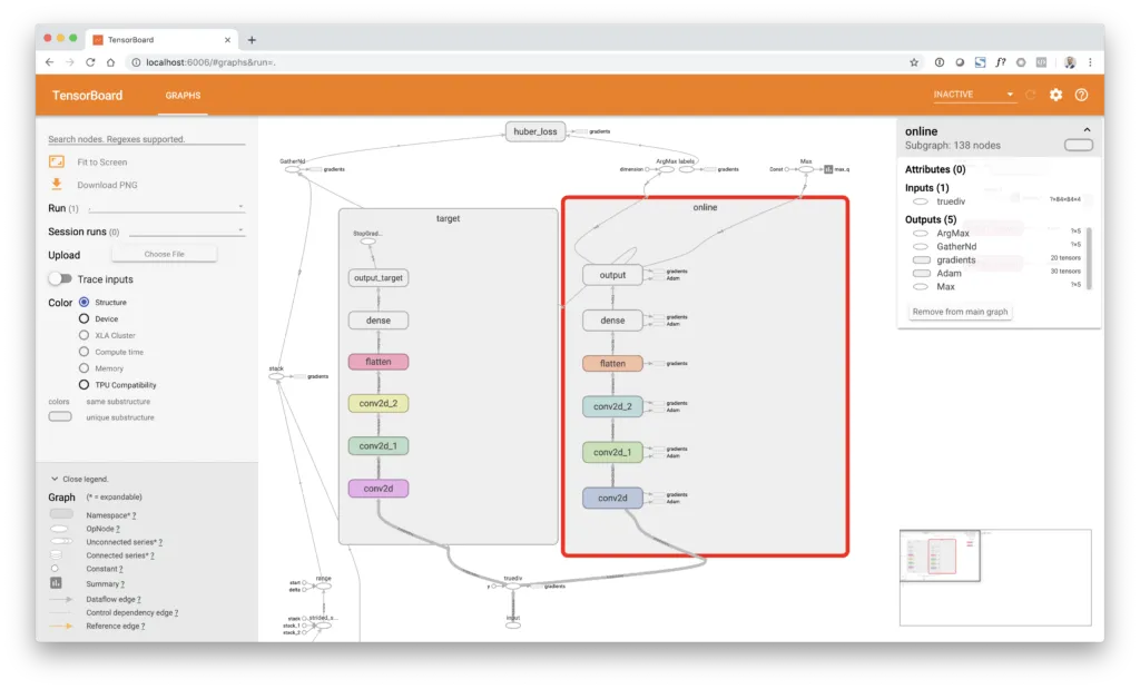
If you take a closer look at the TensorBoard image below, you’ll notice that the model actually consists of not only one but two identical convolutional branches. One is the online network branch, the other one is the target network branch. The online network is acutally trained using gradient descent. The target network is not directly trained but periodically synchronized every copy = 10000 steps by copying the weights from the online branch to the target branch of the network. The target network branch is excluded from gradient descent training by using the tf.stop_gradient() function around the output layer of the branch. This causes a stop in the flow of gradients at the output layer so that they cannot propagate along the branch and so the weights are not updated.
The agent learns by (1) taking random samples of historical transitions, (2) computing the “true” Q-values based on the states of the environment after action, next_state, using the target network branch and the double Q-learning rule, (3) discounting the target Q-values using gamma = 0.9 and (4) run a batch gradient descent step based on the network’s internal Q-prediction and the true Q-values, supplied by target_q. In order to speed up the training process, the agent is not trained after each action but every train_each = 3 frames which corresponds to a training every 4 frames. In addition, not every frame is stored in the replay buffer but each 4th frame. This is called frame skipping. More specifically, a max pooling operation is performed that aggregates the information between the last 4 consecutive frames. This is motivated by the fact that consecutive frames contain nearly the same information which does not add new information to the learning problem and might introduce strongly autocorrelated datapoints.
Speaking of correlated data: our network is trained using adaptive moment estimation (ADAM) and gradient descent at a learning_rate = 0.00025, which requires i.i.d. datapoints in order to work well. This means, that we cannot simply use all new transition tuples subsequently for training since they are highly correlated. To solve this issue we use a concept called experience replay buffer. Hereby, we store every transition of our game in a ring buffer object (in Python the deque() function) which is then randomly sampled from, when we acquire our training data of batch_size = 32. By using a random sampling strategy and a large enough replay buffer, we can assume that the resulting datapoints are (hopefully) not correlated. The following codebox shows the DQNAgent class.
import time
import random
import numpy as np
from collections import deque
import tensorflow as tf
from matplotlib import pyplot as plt


class DQNAgent:
    """ DQN agent """
    def __init__(self, states, actions, max_memory, double_q):
        self.states = states
        self.actions = actions
        self.session = tf.Session()
        self.build_model()
        self.saver = tf.train.Saver(max_to_keep=10)
        self.session.run(tf.global_variables_initializer())
        self.saver = tf.train.Saver()
        self.memory = deque(maxlen=max_memory)
        self.eps = 1
        self.eps_decay = 0.99999975
        self.eps_min = 0.1
        self.gamma = 0.90
        self.batch_size = 32
        self.burnin = 100000
        self.copy = 10000
        self.step = 0
        self.learn_each = 3
        self.learn_step = 0
        self.save_each = 500000
        self.double_q = double_q

    def build_model(self):
        """ Model builder function """
        self.input = tf.placeholder(dtype=tf.float32, shape=(None, ) + self.states, name='input')
        self.q_true = tf.placeholder(dtype=tf.float32, shape=[None], name='labels')
        self.a_true = tf.placeholder(dtype=tf.int32, shape=[None], name='actions')
        self.reward = tf.placeholder(dtype=tf.float32, shape=[], name='reward')
        self.input_float = tf.to_float(self.input) / 255.
        # Online network
        with tf.variable_scope('online'):
            self.conv_1 = tf.layers.conv2d(inputs=self.input_float, filters=32, kernel_size=8, strides=4, activation=tf.nn.relu)
            self.conv_2 = tf.layers.conv2d(inputs=self.conv_1, filters=64, kernel_size=4, strides=2, activation=tf.nn.relu)
            self.conv_3 = tf.layers.conv2d(inputs=self.conv_2, filters=64, kernel_size=3, strides=1, activation=tf.nn.relu)
            self.flatten = tf.layers.flatten(inputs=self.conv_3)
            self.dense = tf.layers.dense(inputs=self.flatten, units=512, activation=tf.nn.relu)
            self.output = tf.layers.dense(inputs=self.dense, units=self.actions, name='output')
        # Target network
        with tf.variable_scope('target'):
            self.conv_1_target = tf.layers.conv2d(inputs=self.input_float, filters=32, kernel_size=8, strides=4, activation=tf.nn.relu)
            self.conv_2_target = tf.layers.conv2d(inputs=self.conv_1_target, filters=64, kernel_size=4, strides=2, activation=tf.nn.relu)
            self.conv_3_target = tf.layers.conv2d(inputs=self.conv_2_target, filters=64, kernel_size=3, strides=1, activation=tf.nn.relu)
            self.flatten_target = tf.layers.flatten(inputs=self.conv_3_target)
            self.dense_target = tf.layers.dense(inputs=self.flatten_target, units=512, activation=tf.nn.relu)
            self.output_target = tf.stop_gradient(tf.layers.dense(inputs=self.dense_target, units=self.actions, name='output_target'))
        # Optimizer
        self.action = tf.argmax(input=self.output, axis=1)
        self.q_pred = tf.gather_nd(params=self.output, indices=tf.stack([tf.range(tf.shape(self.a_true)[0]), self.a_true], axis=1))
        self.loss = tf.losses.huber_loss(labels=self.q_true, predictions=self.q_pred)
        self.train = tf.train.AdamOptimizer(learning_rate=0.00025).minimize(self.loss)
        # Summaries
        self.summaries = tf.summary.merge([
            tf.summary.scalar('reward', self.reward),
            tf.summary.scalar('loss', self.loss),
            tf.summary.scalar('max_q', tf.reduce_max(self.output))
        ])
        self.writer = tf.summary.FileWriter(logdir='./logs', graph=self.session.graph)

    def copy_model(self):
        """ Copy weights to target network """
        self.session.run([tf.assign(new, old) for (new, old) in zip(tf.trainable_variables('target'), tf.trainable_variables('online'))])

    def save_model(self):
        """ Saves current model to disk """
        self.saver.save(sess=self.session, save_path='./models/model', global_step=self.step)

    def add(self, experience):
        """ Add observation to experience """
        self.memory.append(experience)

    def predict(self, model, state):
        """ Prediction """
        if model == 'online':
            return self.session.run(fetches=self.output, feed_dict={self.input: np.array(state)})
        if model == 'target':
            return self.session.run(fetches=self.output_target, feed_dict={self.input: np.array(state)})

    def run(self, state):
        """ Perform action """
        if np.random.rand() < self.eps:
            # Random action
            action = np.random.randint(low=0, high=self.actions)
        else:
            # Policy action
            q = self.predict('online', np.expand_dims(state, 0))
            action = np.argmax(q)
        # Decrease eps
        self.eps *= self.eps_decay
        self.eps = max(self.eps_min, self.eps)
        # Increment step
        self.step += 1
        return action

    def learn(self):
        """ Gradient descent """
        # Sync target network
        if self.step % self.copy == 0:
            self.copy_model()
        # Checkpoint model
        if self.step % self.save_each == 0:
            self.save_model()
        # Break if burn-in
        if self.step < self.burnin:
            return
        # Break if no training
        if self.learn_step < self.learn_each:
            self.learn_step += 1
            return
        # Sample batch
        batch = random.sample(self.memory, self.batch_size)
        state, next_state, action, reward, done = map(np.array, zip(*batch))
        # Get next q values from target network
        next_q = self.predict('target', next_state)
        # Calculate discounted future reward
        if self.double_q:
            q = self.predict('online', next_state)
            a = np.argmax(q, axis=1)
            target_q = reward + (1. - done) * self.gamma * next_q[np.arange(0, self.batch_size), a]
        else:
            target_q = reward + (1. - done) * self.gamma * np.amax(next_q, axis=1)
        # Update model
        summary, _ = self.session.run(fetches=[self.summaries, self.train],
                                      feed_dict={self.input: state,
                                                 self.q_true: np.array(target_q),
                                                 self.a_true: np.array(action),
                                                 self.reward: np.mean(reward)})
        # Reset learn step
        self.learn_step = 0
        # Write
        self.writer.add_summary(summary, self.step)
Training the agent to play
First, we need to instantiate the environment. Here, we use the first level of Super Mario Bros, SuperMarioBros-1-1-v0 as well as a discrete event space with RIGHT_ONLY action space. Additionally, we use a wrapper that applies frame resizing, stacking and max pooling, reward clipping as well as lazy frame loading to the environment.
When the training starts, the agent begins to explore the environment by taking random actions. This is done in order to build up initial experience that serves as a starting point for the actual learning process. After burin = 100000 game frames, the agent slowly starts to replace random actions by actions determined by the CNN policy. This is called an epsilon-greedy policy. Epsilon-greeedy means, that the agent takes a random action with probability epsilon or a policy-based action with probability (1-epsilon). Here, epsilon diminisches linearly during training by a factor of eps_decay = 0.99999975 until it reaches eps = 0.1 where it remains constant for the rest of the training process. It is important to not completely eliminate random actions from the training process in order to avoid getting stuck on locally optimal solutions.
For each action taken, the environment returns a four objects: (1) the next game state, (2) the reward for taking the action, (3) a flag if the episode is done and (4) an info dictionary containing additional information from the environment. After taking the action, a tuple of the returned objects is added to the replay buffer and the agent performs a learning step. After learning, the current state is updated with the next_state and the loop increments. The while loop breaks, if the done flag is True. This corresponds to either the death of Mario or to a successful completion of the level. Here, the agent is trained in 10000 episodes.
import time
import numpy as np
from nes_py.wrappers import BinarySpaceToDiscreteSpaceEnv
import gym_super_mario_bros
from gym_super_mario_bros.actions import RIGHT_ONLY
from agent import DQNAgent
from wrappers import wrapper

# Build env (first level, right only)
env = gym_super_mario_bros.make('SuperMarioBros-1-1-v0')
env = BinarySpaceToDiscreteSpaceEnv(env, RIGHT_ONLY)
env = wrapper(env)

# Parameters
states = (84, 84, 4)
actions = env.action_space.n

# Agent
agent = DQNAgent(states=states, actions=actions, max_memory=100000, double_q=True)

# Episodes
episodes = 10000
rewards = []

# Timing
start = time.time()
step = 0

# Main loop
for e in range(episodes):

    # Reset env
    state = env.reset()

    # Reward
    total_reward = 0
    iter = 0

    # Play
    while True:

        # Show env (diabled)
        # env.render()

        # Run agent
        action = agent.run(state=state)

        # Perform action
        next_state, reward, done, info = env.step(action=action)

        # Remember transition
        agent.add(experience=(state, next_state, action, reward, done))

        # Update agent
        agent.learn()

        # Total reward
        total_reward += reward

        # Update state
        state = next_state

        # Increment
        iter += 1

        # If done break loop
        if done or info['flag_get']:
            break

    # Rewards
    rewards.append(total_reward / iter)

    # Print
    if e % 100 == 0:
        print('Episode {e} - +'
              'Frame {f} - +'
              'Frames/sec {fs} - +'
              'Epsilon {eps} - +'
              'Mean Reward {r}'.format(e=e,
                                       f=agent.step,
                                       fs=np.round((agent.step - step) / (time.time() - start)),
                                       eps=np.round(agent.eps, 4),
                                       r=np.mean(rewards[-100:])))
        start = time.time()
        step = agent.step

# Save rewards
np.save('rewards.npy', rewards)
After each game episode, the averagy reward in this episode is appended to the rewards list. Furthermore, different stats such as frames per second and the current epsilon are printed after every 100 episodes.
Replay
During training, the program checkpoints the current network at save_each = 500000 frames and keeps the 10 latest models on disk. I’ve downloaded several model versions during training to my local machine and produced the following video.
It is so awesome to see the learning progress of the agent! The training process took approximately 20 hours on a GPU accelerated VM on Google Cloud.
Summary and outlook
Reinforcement learning is an exciting field in machine learning that offers a wide range of possible applications in science and business likewise. However, the training of reinforcement learning agents is still quite cumbersome and often requires tedious tuning of hyperparameters and network architecture in order to work well. There have been recent advances, such as RAINBOW (a combination of multiple RL learning strategies) that aim at a more robust framework for training reinforcement learning agents but the field is still an area of active research. Besides Q-learning, there are many other interesting training concepts in reinforcement learning that have been developed. If you want to try different RL agents and training approaches, I suggest you check out Stable Baselines, a great way to easily use state-of-the-art RL agents and training concepts.
If you are a deep learning beginner and want to learn more, you should check our brandnew STATWORX Deep Learning Bootcamp, a 5-day in-person introduction into the field that covers everything you need to know in order to develop your first deep learning models: neural net theory, backpropagation and gradient descent, programming models in Python, TensorFlow and Keras, CNNs and other image recognition models, recurrent networks and LSTMs for time series data and NLP as well as advanced topics such as deep reinforcement learning and GANs.
If you have any comments or questions on my post, feel free to contact me! Also, feel free to use my code (link to GitHub repo) or share this post with your peers on social platforms of your choice.
If you’re interested in more content like this, join our mailing list, constantly bringing you fresh data science, machine learning and AI reads and treats from me and my team at STATWORX right into your inbox!
Lastly, follow me on LinkedIn or my company STATWORX on Twitter, if you’re interested in more!


