Methods Introduction: Statistics with lions - Part 3


Main analysis
Our archaeologists are facing their analytical goal, the prerequisite test of ANOVA has been overcome. To remind you once again of the research question:
H1: The longer the lions are involved in circus games, the higher their weight.
Since all data (weight as a metric and months in the circus as a categorical variable) is prepared, we can get started straight away. The Stata command for the analysis is:
anova gewicht monate_kat
and generates the results below.

Overall, N = 517 cases are available for the analysis, the explained variance proportion is $R^2$ = 0.7505 = 75.05%. The categorized months can therefore explain a very high proportion of variance in weight. Below follows a row for Model and a row for the months. Both rows are the same in this simple model regarding the values (SS stands for Sum of Squares). For SPSS users, it should be noted here that only one of the two rows is listed and labeled as "between groups". Especially the English term is very common in the statistical world and should have also been used by Stata. The "residuals" row is called "within groups" in SPSS, and here too the English technical term is quite common in German literature.
Additionally, the F-value and the associated significance value are indicated for the between-effect. This is significant with $p le .001$ , so the months in the circus have a significant effect on weight. A statement about which categories of months are precisely significant and what difference they have regarding weight cannot be made at this point. The result of the ANOVA is documented with F(df1,df2) = F-value, p-value. In our case with F(5,511) = 311.49, $p le .001$.
In some disciplines, it is customary to specify the effect size of the analysis. Without going into the meaning of this measure in more detail, it should be briefly said here that an effect size makes a statement about whether a found relationship in an analysis also has practical relevance. For ANOVA, $eta^2$ can be easily calculated as the effect size:
$eta^2 = frac{ SS_{between} }{ SS_{top} } = frac{415662.19} {552039.08} = 0.753$
In a one-factor ANOVA like this, $eta^2$ can simply be multiplied by 100, and it holds:
$R^2 = eta^2$
Thus, the interpretation of $eta^2$ can also be easily broken down to the correlation coefficient r, which is simply calculated with
$r = sqrt{R^2} = 0.868$
(Field 2013: 472). Again, the extremely strong effect of the ANOVA is shown. Stata can also calculate the effect size directly after ANOVA, for this the following command must be used
estat esize
Since $eta^2$ mathematically has a bias (Levine 2002), Omega squared is often given as the measure of effect size for an ANOVA. Stata can now calculate this natively with
estat esize, omega
The result is $omega^2 = 0.7502$, regarding the limits, the same applies as for $eta^2$ (Kirk 1996). So there is a strong effect. But how do the months differ in detail?
posthoc-Test
To remind you how heavy the lions are on average in the individual month categories, the table from part 2 is shown here again.

Stata offers several posthoc commands following ANOVA. With
pwcompare monate_kat, group effects mcompare(bon)all month categories, i.e., all possible combinations, would be compared with each other. This generates quite a large table, which is not displayed here as it is not of interest to us. Since the goal of the researchers was to investigate whether lions gain weight during longer stays in circus games, we are currently only interested in whether lions in the next higher category of months differ from the previous category. The command "pwcompare" cannot help us here, so we now have to perform
contrast ar.monate_kat, mcompare(bon) effectsWith the prefix “ar.” we instruct Stata to always compare from the first category (less than 6 months) to the next higher category. The results are found in the table below.
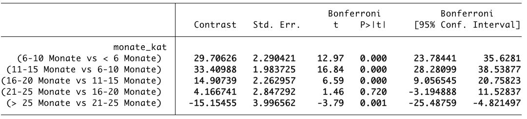
The category "6-10 months" differs from the category "$le$ 6 months" by 29.71. The contrast is nothing other than the difference in the means of these categories, i.e., 131.17 – 101.46 = 29.71. The last mentioned category of the contrast is always subtracted from the first mentioned category. Since the value is positive, this means that lions with 6-10 months in the circus are on average 29.71kg heavier than lions that are less than 6 months in the circus. This result is significant with t = 12.97, $p le .001$. Bonferroni was performed as the posthoc test. A discussion of the countless tests cannot be given here, and reference should be made to further technical literature (Field 2013: 458 ff.). Even though Bonferroni calculates quite conservatively, it can be said with regard to this analysis that no other test method yields a different result.
The look at the table reveals that lions become heavier with increasing months, initially gaining 29.71kg ($p le .001$), then 33.41kg ($p le .001$), the weight gain then decreases to 14.91kg ($p le .001$) when comparing "16-20 months" vs. "11-15 months", and in the subsequent comparison the gain is only on average 4.17kg but is not significant with p = .720. In the comparison of the last and penultimate category with each other, the lions then lose weight again, the contrast is -15.15 ($p le .01$).
With the help of the comfortable command "margins" or "marginsplot", the following graphic can now be displayed regarding this change, where the code, despite the simplicity of the representation, is relatively long and should be omitted here.

Although the above graphic already fulfills the wishes of the researchers in terms of content, another one should be generated (see below). This graphic shows the value of the contrast between the ascending categories of months. Additionally, a red line was drawn at the value for 0kg, which is once broken through by the confidence interval. At "21-25 vs. 16-20" months, the contrast is +4.17kg, so there is still a slight weight gain, the confidence interval, however, lies between -3.20 and +11.53. With a 95% probability, the contrast lies in this range and encompasses the value 0. The result is thus not significant even without knowing the actual p-values, as the contrast can also be negative instead of positive (+4.17kg) (up to -3.20kg), and the substantive interpretation would be completely different.

The researchers see their hypothesis as largely confirmed but ask themselves after the initial euphoria whether the age of the lions might have a side effect, which is called a covariate in statistical terms and leads to a covariance analysis (ANCOVA).
References
- Cohen, J. (1988): Statistical Power Analysis for the Behavioral Sciences. Hoboken: Taylor and Francis
- Field, Andy (2013): Discovering Statistics Using SPSS. 4th Edition, SAGE: London
- Kirk, R. E. (1996): Practical significance: A concept whose time has come. Educational and Psychological Measurement 56(5), S. 746-759
- Levine, T. R., & Hullett, C. R. (2002). Eta Squared, Partial Eta Squared, and Misreporting of Effect Size in Communication Research. Human Communication Research 28(4), S. 612–625


