Methods Introduction: Statistics with Lions – Part 2


After the descriptive examination of the historical data, our archaeologists take a step further and pose the following research question:
H1: The longer the lions are engaged in circus games, the higher their weight.
To answer this question, the researchers initially use a simple correlation analysis.
This reveals that weight and months in the circus are positively correlated with Pearson’s Rho $rho$ = .7718 and a significance of p $le$ .001. Thus, the lions gained weight the longer they were in the circus.
pwcorr weight months, sig obsHowever, the evaluating statisticians knew from the previous analysis that the weight gain did not progress continuously. Especially for lions that had been in the circus for a longer time, it could be graphically seen that their weight decreased again. Therefore, the scientists categorized the months to perform a variance analysis (ANOVA) with the new variable.
tab months_kat
The goal of ANOVA now is to see if the average weight between the newly formed groups is different, and (advantage ANOVA over correlation) in which direction the weight differs. The procedure imposes several requirements on the data, which are to be considered individually in part 2 of this series.
Prerequisites of an ANOVA
Assumption 1: The dependent variable (weight) should be metric. Weight corresponds to a ratio scale due to its zero point.
Assumption 2: The independent variable (months in categories) should consist of at least 3 categories. Our variable consists of a total of 6 categories and thus seems ideally suited.
Assumption 3: Independent observations should be present. This means that no relationship should exist between the observations in and between each group.
While the first three assumptions cannot be checked with a statistical procedure, this is the case with the now following assumptions.
Assumption 4: No significant outliers should exist. The verification of this assumption is done graphically with the help of boxplots. As you can see below, statistically speaking, there are none, as otherwise points would be present above or below the antennas in the representation.
graph box weight, over(months_kat, label(labsize(vsmall)))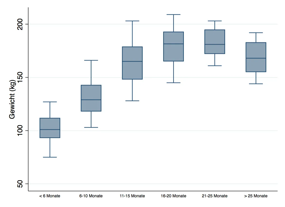
Statistically speaking, calculating outliers is very simple: Starting from the upper and lower end of the box (75% and 25% quartile), the interquartile range (for each group) is calculated.
Formula: $IQR = x_{0.75} – x_{0.25}$
For the lions that have been in the circus for less than 6 months, this can be calculated with the Stata command:
centile weight if months_kat == 1, centile(25 75)
So the 75% quartile in this group is 112kg, and the 25% quartile is 93kg. The IQR is thus 112kg - 93kg = 19kg.
An outlier "upwards" or "downwards" is defined such that 1.5 times the edge length must not be exceeded. This is considered the standard value in the calculation of outliers, so the end of the antennas in the boxplot represents exactly this threshold. This is calculated with:
$Outliers_{upwards} = |{frac{ Wert - Quartil_{0,75} }{ IQR } }|Outliers_{downwards} = |{frac{ Wert - Quartil_{0,25} }{ IQR } }| $
Using the example of lions in category 1 (less than 6 months in the circus), let's display the minimum and maximum weight.
su gewicht if monate_kat == 1
The minimum weight of these lions is 75kg, and the maximum weight is 127kg. The proportion of the IQR is thus:
$Outliers_{upwards} = |{frac{ 127 - 112 }{ 19 } }| = 0.789 le 1.5 Outliers_{downwards} = |{frac{ 75 - 93 }{ 19 } }| = 0.947 le 1.5 $
Since the minimum and maximum in this group do not exceed the value of 1.5, no outliers are present. Unfortunately, Stata does not natively provide a calculation including the display of outliers according to this logic, but the command "extremes" can be additionally installed. The command performs the calculations just discussed immediately and would display outlier values.
ssc install extremes
bysort months_kat: extreme weight, iqr(1.5)
Since entering the command, grouped by the categories of months, shows no values, the graphical consideration of the boxplots is naturally confirmed.
Assumption 5: The dependent variable (weight) should be normally distributed within each category (months). Normal distribution is often considered a casus belli for the further course of the analysis. Almost stoically, the rather not recommended Kolmogorov-Smirnov test (Field 184 ff.) is often used exclusively for this purpose, without also looking at the graphical distribution itself. The histograms below consider the distribution of weight across all 6 categories of months and also give the result of the recommended Shapiro-Wilk test for normal distribution. If the significance p $le$.05 in this test (similar to Kolmogorov-Smirnov), the variable can be considered normally distributed.

For three of the six categories, the test with p $le$.05 indicates that there is no normal distribution. Visually, however, no gross violation can be detected in these 3 categories either, so there is no objection to the evaluation with ANOVA here. Furthermore, reference is made to the numerous literature on the robustness of ANOVA in violation of this assumption.
Assumption 6: The last assumption of ANOVA is that the variances between groups concerning the dependent variable are equal. This is also known as homogeneity of variances. With a sole focus on variance, this can hardly be assessed (see lower table), so a test for variance homogeneity must be performed.
tabstat weight, statistics(mean var) by(months_kat)
This test is the Levene test, which proves variance homogeneity with p $ge$ .05 and is requested in Stata via
robvar weight, by(months_kat)
The output of the Levene test is marked in Stata with W0 and shows p $le$.001 in this case, so homogeneity of variances cannot be spoken of. In this case, a correction per Welch or Brown-Forsythe should be made for the calculation of the F-values of ANOVA, and posthoc tests for the violation of this assumption also exist. Unlike SPSS, Stata does not have an option within the command to apply Welch or Brown-Forsythe, but reference is also made to the robustness of ANOVA here. Additionally, Stata, with the help of the regression command, which can be used complementary to ANOVA, has far greater possibilities of calculation when this problem arises. For our analysts, the violation of variance homogeneity is currently not an issue.
A Word
The assumptions of ANOVA are often considered sacred and immutable law. Often, when an assumption is violated, to which ANOVA reacts quite robustly, a non-parametric alternative procedure is used. Moreover, not infrequently, means over the groups are presented descriptively and then interpreted with the results (significances) of the non-parametric procedure. Overall, ANOVA is a robust procedure that can still be applied even in the face of gross violations of the assumptions.
References
- Field, Andy (2013): Discovering Statistics Using SPSS, 4th Edition. SAGE: London


