Text classification is one of the most common applications of natural language processing (NLP). It is the task of assigning a set of predefined categories to a text snippet. Depending on the type of problem, the text snippet could be a sentence, a paragraph, or even a whole document. There are many potential real-world applications for text classification, but among the most common ones are sentiment analysis, topic modeling and intent, spam, and hate speech detection.
The standard approach to text classification is training a classifier in a supervised regime. To do so, one needs pairs of text and associated categories (aka labels) from the domain of interest as training data. Then, any classifier (e.g., a neural network) can learn a mapping function from the text to the most likely category. While this approach can work quite well for many settings, its feasibility highly depends on the availability of those hand-labeled pairs of training data.
Though pre-trained language models like BERT can reduce the amount of data needed, it does not make it obsolete altogether. Therefore, for real-world applications, data availability remains the biggest hurdle.
Zero-Shot Learning
Though there are various definitions of zero-shot learning1, it can broadly speaking be defined as a regime in which a model solves a task it was not explicitly trained on before.
It is important to understand, that a “task” can be defined in both a broader and a narrower sense: For example, the authors of GPT-2 showed that a model trained on language generation can be applied to entirely new downstream tasks like machine translation2. At the same time, a narrower definition of task would be to recognize previously unseen categories in images as shown in the OpenAI CLIP paper3.
But what all these approaches have in common is the idea of extrapolation of learned concepts beyond the training regime. A powerful concept, because it disentangles the solvability of a task from the availability of (labeled) training data.
Zero-Shot Learning for Text Classification
Solving text classification tasks with zero-shot learning can serve as a good example of how to apply the extrapolation of learned concepts beyond the training regime. One way to do this is using natural language inference (NLI) as proposed by Yin et al. (2019)4. There are other approaches as well like the calculation of distances between text embeddings or formulating the problem as a cloze
In NLI the task is to determine whether a hypothesis is true (entailment), false (contradiction), or undetermined (neutral) given a premise5. A typical NLI dataset consists of sentence pairs with associated labels in the following form:
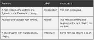
Examples from http://nlpprogress.com/english/natural_language_inference.html
Yin et al. (2019) proposed to use large language models like BERT trained on NLI datasets and exploit their language understanding capabilities for zero-shot text classification. This can be done by taking the text of interest as the premise and formulating one hypothesis for each potential category by using a so-called hypothesis template. Then, we let the NLI model predict whether the premise entails the hypothesis. Finally, the predicted probability of entailment can be interpreted as the probability of the label.
Zero-Shot Text Classification with Hugging Face 🤗
Let’s explore the above-formulated idea in more detail using the excellent Hugging Face implementation for zero-shot text classification.
We are interested in classifying the sentence below into pre-defined topics:
topics = ['Web', 'Panorama', 'International', 'Wirtschaft', 'Sport', 'Inland', 'Etat', 'Wissenschaft', 'Kultur']
test_txt = 'Eintracht Frankfurt gewinnt die Europa League nach 6:5-Erfolg im Elfmeterschießen gegen die Glasgow Rangers'
Thanks to the 🤗 pipeline abstraction, we do not need to define the prediction task ourselves. We just need to instantiate a pipeline and define the task as zero-shot-text-classification. The pipeline will take care of formulating the premise and hypothesis as well as deal with the logits and probabilities from the model.
As written above, we need a language model that was pre-trained on an NLI task. The default model for zero-shot text classification in 🤗 is bart-large-mnli. BART is a transformer encoder-decoder for sequence-2-sequence modeling with a bidirectional (BERT-like) encoder and an autoregressive (GPT-like) decoder6. The mnli suffix means that BART was then further fine-tuned on the MultiNLI dataset7.
But since we are using German sentences and BART is English-only, we need to replace the default model with a custom one. Thanks to the 🤗 model hub, finding a suitable candidate is quite easy. In our case, mDeBERTa-v3-base-xnli-multilingual-nli-2mil7 is such a candidate. Let’s decrypt the name shortly for a better understanding: it is a multilanguage version of DeBERTa-v3-base (which is itself an improved version of BERT/RoBERTa8) that was then fine-tuned on two cross-lingual NLI datasets (XNLI8 and multilingual-NLI-26lang10).
With the correct task and the correct model, we can now instantiate the pipeline:
from transformers import pipeline
model = 'MoritzLaurer/mDeBERTa-v3-base-xnli-multilingual-nli-2mil7'
pipe = pipeline(task='zero-shot-classification', model=model, tokenizer=model)
Next, we call the pipeline to predict the most likely category of our text given the candidates. But as a final step, we need to replace the default hypothesis template as well. This is necessary since the default is again in English. We, therefore, define the template as 'Das Thema is {}'. Note that, {} is a placeholder for the previously defined topic candidates. You can define any template you like as long as it contains a placeholder for the candidates:
template_de = 'Das Thema ist {}'
prediction = pipe(test_txt, topics, hypothesis_template=template_de)
Finally, we can assess the prediction from the pipeline. The code below will output the three most likely topics together with their predicted probabilities:
print(f'Zero-shot prediction for: \n {prediction["sequence"]}')
top_3 = zip(prediction['labels'][0:3], prediction['scores'][0:3])
for label, score in top_3:
    print(f'{label} - {score:.2%}')
Zero-shot prediction for:
Eintracht Frankfurt gewinnt die Europa League nach 6:5-Erfolg im Elfmeterschießen gegen die Glasgow Rangers
Sport - 77.41%
International - 15.69%
Inland - 5.29%As one can see, the zero-shot model produces a reasonable result with “Sport” being the most likely topic followed by “International” and “Inland”.
Below are a few more examples from other categories. Like before, the results are overall quite reasonable. Note how for the second text the model predicts an unexpectedly low probability of “Kultur”.
further_examples = ['Verbraucher halten sich wegen steigender Zinsen und Inflation beim Immobilienkauf zurück',
                    '„Die bitteren Tränen der Petra von Kant“ von 1972 geschlechtsumgewandelt und neu verfilmt',
                    'Eine 541 Millionen Jahre alte fossile Alge weist erstaunliche Ähnlichkeit zu noch heute existierenden Vertretern auf']

for txt in further_examples:
    prediction = pipe(txt, topics, hypothesis_template=template_de)
    print(f'Zero-shot prediction for: \n {prediction["sequence"]}')
    top_3 = zip(prediction['labels'][0:3], prediction['scores'][0:3])
    for label, score in top_3:
        print(f'{label} - {score:.2%}')
Zero-shot prediction for:
Verbraucher halten sich wegen steigender Zinsen und Inflation beim Immobilienkauf zurück
Wirtschaft - 96.11%
Inland - 1.69%
Panorama - 0.70%
Zero-shot prediction for:
„Die bitteren Tränen der Petra von Kant“ von 1972 geschlechtsumgewandelt und neu verfilmt
International - 50.95%
Inland - 16.40%
Kultur - 7.76%
Zero-shot prediction for:
Eine 541 Millionen Jahre alte fossile Alge weist erstaunliche Ähnlichkeit zu noch heute existierenden Vertretern auf
Wissenschaft - 67.52%
Web - 8.14%
Inland - 6.91%The entire code can be found on GitHub. Besides the examples from above, you will find there also applications of zero-shot text classifications on two labeled datasets including an evaluation of the accuracy. In addition, I added some prompt-tuning by playing around with the hypothesis template.
Concluding Thoughts
Zero-shot text classification offers a suitable approach when either training data is limited (or even non-existing) or as an easy-to-implement benchmark for more sophisticated methods. While explicit approaches, like fine-tuning large pre-trained models, certainly still outperform implicit approaches, like zero-shot learning, their universal applicability makes them very appealing.
In addition, we should expect zero-shot learning, in general, to become more important over the next few years. This is because the way we will use models to solve tasks will evolve with the increasing importance of large pre-trained models. Therefore, I advocate that already today zero-shot techniques should be considered part of every modern data scientist’s toolbox.
Sources:
1 https://joeddav.github.io/blog/2020/05/29/ZSL.html
2 https://d4mucfpksywv.cloudfront.net/better-language-models/language_models_are_unsupervised_multitask_learners.pdf
3 https://arxiv.org/pdf/2103.00020.pdf
4 https://arxiv.org/pdf/1909.00161.pdf
5 http://nlpprogress.com/english/natural_language_inference.html
6 https://arxiv.org/pdf/1910.13461.pdf
7 https://huggingface.co/datasets/multi_nli
8 https://arxiv.org/pdf/2006.03654.pdf
9 https://huggingface.co/datasets/xnli
10 https://huggingface.co/datasets/MoritzLaurer/multilingual-NLI-26lang-2mil7
We at work a lot with R and often use the same little helper functions within our projects. These functions ease our daily work life by reducing repetitive code parts or by creating overviews of our projects. To share these functions within our teams and with others as well, I started to collect them and created an R package out of them called . Besides sharing, I also wanted to have some use cases to improve my debugging and optimization skills. With time the package grew, and more and more functions came together. Last time I presented each function as part of an advent calendar. For our new website launch, I combined all of them into this one and will present each current function from the package.
Most functions were developed when there was a problem, and one needed a simple solution. For example, the text shown was too long and needed to be shortened (see evenstrings). Other functions exist to reduce repetitive tasks – like reading in multiple files of the same type (see read_files). Therefore, these functions might be useful to you, too!
You can check out our
1. char_replace
This little helper replaces non-standard characters (such as the German umlaut “ä”) with their standard equivalents (in this case, “ae”). It is also possible to force all characters to lower case, trim whitespaces, or replace whitespaces and dashes with underscores.
Let’s look at a small example with different settings:
x <- " Élizàldë-González Strasse"
char_replace(x, to_lower = TRUE)
[1] "elizalde-gonzalez strasse"char_replace(x, to_lower = TRUE, to_underscore = TRUE)[1] "elizalde_gonzalez_strasse"char_replace(x, to_lower = FALSE, rm_space = TRUE, rm_dash = TRUE)[1] "ElizaldeGonzalezStrasse"
2. checkdir
This little helper checks a given folder path for existence and creates it if needed.
checkdir(path = "testfolder/subfolder")file.exists() and dir.create()
3. clean_gc
This little helper frees your memory from unused objects. Well, basically, it just calls gc() a few times. I used this some time ago for a project where I worked with huge data files. Even though we were lucky enough to have a big server with 500GB RAM, we soon reached its limits. Since we typically parallelize several processes, we needed to preserve every bit and byte of RAM we could get. So, instead of having many lines like this one:
gc();gc();gc();gc()clean_gc() for convenience. Internally, gc()
Some further thoughts
gc() and its usefulness. If you want to learn more about this, I suggest you check out the
4. count_na
This little helper counts missing values within a vector.
x <- c(NA, NA, 1, NaN, 0)
count_na(x)3sum(is.na(x)) counting the NA values. If you want the mean instead of the sum, you can set prop = TRUE
5. evenstrings
This little helper splits a given string into smaller parts with a fixed length. But why? I needed this function while creating a plot with a long title. The text was too long for one line, and I wanted to separate it nicely instead of just cutting it or letting it run over the edges.
Given a long string like…
long_title <- c("Contains the months: January, February, March, April, May, June, July, August, September, October, November, December")split = "," with a maximum length of char = 60
short_title <- evenstrings(long_title, split = ",", char = 60)The function has two possible output formats, which can be chosen by setting newlines = TRUE or FALSE:
- one string with line separators
\n - a vector with each sub-part.
Another use case could be a message that is printed at the console with cat():
cat(long_title)Contains the months: January, February, March, April, May, June, July, August, September, October, November, Decembercat(short_title)Contains the months: January, February, March, April, May,
June, July, August, September, October, November, December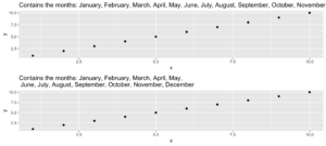
Code for plot example
p1 <- ggplot(data.frame(x = 1:10, y = 1:10),
  aes(x = x, y = y)) +
  geom_point() +
  ggtitle(long_title)

p2 <- ggplot(data.frame(x = 1:10, y = 1:10),
  aes(x = x, y = y)) +
  geom_point() +
  ggtitle(short_title)

multiplot(p1, p2)
6. get_files
This little helper does the same thing as the “Find in files” search within RStudio. It returns a vector with all files in a given folder that contain the search pattern. In your daily workflow, you would usually use the shortcut key SHIFT+CTRL+F. With get_files() you can use this functionality within your scripts.
7. get_network
This little helper aims to visualize the connections between R functions within a project as a flowchart. Herefore, the input is a directory path to the function or a list with the functions, and the outputs are an adjacency matrix and an igraph object. As an example, we use :
net <- get_network(dir = "flowchart/R_network_functions/", simplify = FALSE)
g1 <- net$igraph
Input
There are five parameters to interact with the function:
- A path
dirwhich shall be searched. - A character vector
variationswith the function’s definition string -the default isc(" <- function", "<- function", "<-function"). - A
patterna string with the file suffix – the default is"\\.R$". - A boolean
simplifythat removes functions with no connections from the plot. - A named list
all_scripts, which is an alternative todir. This is mainly just used for testing purposes.
For normal usage, it should be enough to provide a path to the project folder.
Output
The given plot shows the connections of each function (arrows) and also the relative size of the function’s code (size of the points). As mentioned above, the output consists of an adjacency matrix and an igraph object. The matrix contains the number of calls for each function. The igraph object has the following properties:
- The names of the functions are used as label.
- The number of lines of each function (without comments and empty ones) are saved as the size.
- The folder‘s name of the first folder in the directory.
- A color corresponding to the folder.
With these properties, you can improve the network plot, for example, like this:
library(igraph)

# create plots ------------------------------------------------------------
l <- layout_with_fr(g1)
colrs <- rainbow(length(unique(V(g1)$color)))

plot(g1,
     edge.arrow.size = .1,
     edge.width = 5*E(g1)$weight/max(E(g1)$weight),
     vertex.shape = "none",
     vertex.label.color = colrs[V(g1)$color],
     vertex.label.color = "black",
     vertex.size = 20,
     vertex.color = colrs[V(g1)$color],
     edge.color = "steelblue1",
     layout = l)
legend(x = 0,
       unique(V(g1)$folder), pch = 21,
       pt.bg = colrs[unique(V(g1)$color)],
       pt.cex = 2, cex = .8, bty = "n", ncol = 1)
8. get_sequence
This little helper returns indices of recurring patterns. It works with numbers as well as with characters. All it needs is a vector with the data, a pattern to look for, and a minimum number of occurrences.
Let’s create some time series data with the following code.
library(data.table)

# random seed
set.seed(20181221)

# number of observations
n <- 100

# simulationg the data
ts_data <- data.table(DAY = 1:n, CHANGE = sample(c(-1, 0, 1), n, replace = TRUE))
ts_data[, VALUE := cumsum(CHANGE)]
This is nothing more than a random walk since we sample between going down (-1), going up (1), or staying at the same level (0). Our time series data looks like this:
Assume we want to know the date ranges when there was no change for at least four days in a row.
ts_data[, get_sequence(x = CHANGE, pattern = 0, minsize = 4)] min max
[1,] 45 48
[2,] 65 69We can also answer the question if the pattern “down-up-down-up” is repeating anywhere:
ts_data[, get_sequence(x = CHANGE, pattern = c(-1,1), minsize = 2)] min max
[1,] 88 91geom_rect

Code for the plot
rect <- data.table(
  rbind(ts_data[, get_sequence(x = CHANGE, pattern = c(0), minsize = 4)],
        ts_data[, get_sequence(x = CHANGE, pattern = c(-1,1), minsize = 2)]),
  GROUP = c("no change","no change","down-up"))

ggplot(ts_data, aes(x = DAY, y = VALUE)) +
  geom_line() +
  geom_rect(data = rect,
  inherit.aes = FALSE,
  aes(xmin = min - 1,
  xmax = max,
  ymin = -Inf,
  ymax = Inf,
  group = GROUP,
  fill = GROUP),
  color = "transparent",
  alpha = 0.5) +
  scale_fill_manual(values = statworx_palette(number = 2, basecolors = c(2,5))) +
  theme_minimal()
9. intersect2
This little helper returns the intersect of multiple vectors or lists. I found this function , thought it is quite useful and adjusted it a bit.
intersect2(list(c(1:3), c(1:4)), list(c(1:2),c(1:3)), c(1:2))[1] 1 2Internally, the problem of finding the intersection is solved recursively, if an element is a list and then stepwise with the next element.
10. multiplot
This little helper combines multiple ggplots into one plot. This is a function taken from .
An advantage over facets is, that you don’t need all data for all plots within one object. Also you can freely create each single plot – which can sometimes also be a disadvantage.
With the layout parameter you can arrange multiple plots with different sizes. Let’s say you have three plots and want to arrange them like this:
1    2    2
1    2    2
3 3 3multiplot
multiplot(plotlist = list(p1, p2, p3),
          layout = matrix(c(1,2,2,1,2,2,3,3,3), nrow = 3, byrow = TRUE))
Code for plot example
# star coordinates
c1  =   cos((2*pi)/5)
c2  =   cos(pi/5)
s1  =   sin((2*pi)/5)
s2  =   sin((4*pi)/5)

data_star <- data.table(X = c(0, -s2, s1, -s1, s2),
                        Y = c(1, -c2, c1, c1, -c2))

p1 <- ggplot(data_star, aes(x = X, y = Y)) +
  geom_polygon(fill = "gold") +
  theme_void()

# tree
set.seed(24122018)
n <- 10000
lambda <- 2
data_tree <- data.table(X = c(rpois(n, lambda), rpois(n, 1.1*lambda)),
                        TYPE = rep(c("1", "2"), each = n))
data_tree <- data_tree[, list(COUNT = .N), by = c("TYPE", "X")]
data_tree[TYPE == "1", COUNT := -COUNT]

p2 <- ggplot(data_tree, aes(x = X, y = COUNT, fill = TYPE)) +
  geom_bar(stat = "identity") +
  scale_fill_manual(values = c("green", "darkgreen")) +
  coord_flip() +
  theme_minimal()

# gifts
data_gifts <- data.table(X = runif(5, min = 0, max = 10),
                         Y = runif(5, max = 0.5),
                         Z = sample(letters[1:5], 5, replace = FALSE))

p3 <- ggplot(data_gifts, aes(x = X, y = Y)) +
  geom_point(aes(color = Z), pch = 15, size = 10) +
  scale_color_brewer(palette = "Reds") +
  geom_point(pch = 12, size = 10, color = "gold") +
  xlim(0,8) +
  ylim(0.1,0.5) +
  theme_minimal() +
  theme(legend.position="none")
11. na_omitlist
This little helper removes missing values from a list.
y <- list(NA, c(1, NA), list(c(5:6, NA), NA, "A"))There are two ways to remove the missing values, either only on the first level of the list or wihtin each sub level.
na_omitlist(y, recursive = FALSE)[[1]]
[1] 1 NA
[[2]]
[[2]][[1]]
[1] 5 6 NA
[[2]][[2]]
[1] NA
[[2]][[3]]
[1] "A"na_omitlist(y, recursive = TRUE)[[1]]
[1] 1
[[2]]
[[2]][[1]]
[1] 5 6
[[2]][[2]]
[1] "A"12. %nin%
%in%
all.equal( c(1,2,3,4) %nin% c(1,2,5),
          !c(1,2,3,4) %in%  c(1,2,5))
[1] TRUE.
13. object_size_in_env
This little helper shows a table with the size of each object in the given environment.
If you are in a situation where you have coded a lot and your environment is now quite messy, object_size_in_env helps you to find the big fish with respect to memory usage. Personally, I ran into this problem a few times when I looped over multiple executions of my models. At some point, the sessions became quite large in memory and I did not know why! With the help of object_size_in_env and some degubbing I could locate the object that caused this problem and adjusted my code accordingly.
First, let us create an environment with some variables.
# building an environment
this_env <- new.env()
assign("Var1", 3, envir = this_env)
assign("Var2", 1:1000, envir = this_env)
assign("Var3", rep("test", 1000), envir = this_env)format(object.size()) is used. With the unit the output format can be changed (eg. "B", "MB" or "GB"
# checking the size
object_size_in_env(env = this_env, unit = "B")
OBJECT SIZE UNIT
1: Var3 8104 B
2: Var2 4048 B
3: Var1 56 B14. print_fs
This little helper returns the folder structure of a given path. With this, one can for example add a nice overview to the documentation of a project or within a git. For the sake of automation, this function could run and change parts wihtin a log or news file after a major change.
If we take a look at the same example we used for the get_network function, we get the following:
print_fs("~/flowchart/", depth = 4)1 flowchart
2 ¦--create_network.R
3 ¦--getnetwork.R
4 ¦--plots
5 ¦ ¦--example-network-helfRlein.png
6 ¦ °--improved-network.png
7 ¦--R_network_functions
8 ¦ ¦--dataprep
9 ¦ ¦ °--foo_01.R
10 ¦ ¦--method
11 ¦ ¦ °--foo_02.R
12 ¦ ¦--script_01.R
13 ¦ °--script_02.R
14 °--README.md With depth we can adjust how deep we want to traverse through our folders.
15. read_files
This little helper reads in multiple files of the same type and combines them into a data.table. Which kind of file reading function should be used can be choosen by the FUN argument.
If you have a list of files, that all needs to be loaded in with the same function (e.g. read.csv), instead of using lapply and rbindlist now you can use this:
read_files(files, FUN = readRDS)
read_files(files, FUN = readLines)
read_files(files, FUN = read.csv, sep = ";")
Internally, it just uses lapply and rbindlist but you dont have to type it all the time. The read_files combines the single files by their column names and returns one data.table. Why data.table? Because I like it. But, let’s not go down the rabbit hole of data.table vs dplyr ().
16. save_rds_archive
This little helper is a wrapper around base R saveRDS() and checks if the file you attempt to save already exists. If it does, the existing file is renamed / archived (with a time stamp), and the “updated” file will be saved under the specified name. This means that existing code which depends on the file name remaining constant (e.g., readRDS() calls in other scripts) will continue to work while an archived copy of the – otherwise overwritten – file will be kept.
17. sci_palette
This little helper returns a set of colors which we often use at statworx. So, if – like me – you cannot remeber each hex color code you need, this might help. Of course these are our colours, but you could rewrite it with your own palette. But the main benefactor is the plotting method – so you can see the color instead of only reading the hex code.
To see which hex code corresponds to which colour and for what purpose to use it
sci_palette(scheme = "new")Tech Blue Black White Light Grey Accent 1 Accent 2 Accent 3
"#0000FF" "#000000" "#FFFFFF" "#EBF0F2" "#283440" "#6C7D8C" "#B6BDCC"
Highlight 1 Highlight 2 Highlight 3
"#00C800" "#FFFF00" "#FE0D6C"
attr(,"class")
[1] "sci"plot()
plot(sci_palette(scheme = "new"))

18. statusbar
This little helper prints a progress bar into the console for loops.
There are two nessecary parameters to feed this function:
runis either the iterator or its numbermax.runis either all possible iterators in the order they are processed or the maximum number of iterations.
So for example it could be run = 3 and max.run = 16 or run = "a" and max.run = letters[1:16].
Also there are two optional parameter:
percent.maxinfluences the width of the progress barinfois an additional character, which is printed at the end of the line. By default it isrun.
A little disadvantage of this function is, that it does not work with parallel processes. If you want to have a progress bar when using apply functions check out .
19. statworx_palette
This little helper is an addition to yesterday’s . We picked colors 1, 2, 3, 5 and 10 to create a flexible color palette. If you need 100 different colors – say no more!
In contrast to sci_palette() the return value is a character vector. For example if you want 16 colors:
statworx_palette(16, scheme = "old")[1] "#013848" "#004C63" "#00617E" "#00759A" "#0087AB" "#008F9C" "#00978E" "#009F7F"
[9] "#219E68" "#659448" "#A98B28" "#ED8208" "#F36F0F" "#E45A23" "#D54437" "#C62F4B"If we now plot those colors, we get this nice rainbow like gradient.
library(ggplot2)

ggplot(plot_data, aes(x = X, y = Y)) +
  geom_point(pch = 16, size = 15, color = statworx_palette(16, scheme = "old")) +
  theme_minimal()
reorder parameter, which samples the color’s order so that neighbours might be a bit more distinguishable. Also if you want to change the used colors, you can do so with basecolors
ggplot(plot_data, aes(x = X, y = Y)) +
  geom_point(pch = 16, size = 15,
             color = statworx_palette(16, basecolors = c(4,8,10), scheme = "new")) +
  theme_minimal()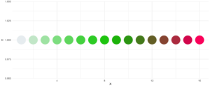
20. strsplit
This little helper adds functionality to the base R function strsplit – hence the same name! It is now possible to split before, after or between a given delimiter. In the case of between you need to specify two delimiters.
An earlier version of this function can be found , where I describe the used regular expressions, if you are interested.
Here is a little example on how to use the new strsplit.
text <- c("This sentence should be split between should and be.")

strsplit(x = text, split = " ")
strsplit(x = text, split = c("should", " be"), type = "between")
strsplit(x = text, split = "be", type = "before")
[[1]]
[1] "This" "sentence" "should" "be" "split" "between" "should" "and"
[9] "be."
[[1]]
[1] "This sentence should" " be split between should and be."
[[1]]
[1] "This sentence should " "be split " "between should and "
[4] "be."21. to_na
This little helper is just a convenience function. Some times during your data preparation, you have a vector with infinite values like Inf or -Inf or even NaN values. Thos kind of value can (they do not have to!) mess up your evaluation and models. But most functions do have a tendency to handle missing values. So, this little helper removes such values and replaces them with NA.
A small exampe to give you the idea:
test <- list(a = c("a", "b", NA),
             b = c(NaN, 1,2, -Inf),
             c = c(TRUE, FALSE, NaN, Inf))

lapply(test, to_na)
$a
[1] "a" "b" NA
$b
[1] NA 1 2 NA
$c
[1] TRUE FALSE NA Since there are different types of NA depending on the other values within a vector. You might want to check the format if you do to_na
test <- list(NA, c(NA, "a"), c(NA, 2.3), c(NA, 1L))
str(test)
List of 4
$ : logi NA
$ : chr [1:2] NA "a"
$ : num [1:2] NA 2.3
$ : int [1:2] NA 122. trim
This little helper removes leading and trailing whitespaces from a string. With trimws was introduced, which does the exact same thing. This just shows, it was not a bad idea to write such a function. 😉
x <- c("  Hello world!", "  Hello world! ", "Hello world! ")
trim(x, lead = TRUE, trail = TRUE)
[1] "Hello world!" "Hello world!" "Hello world!"The lead and trail parameters indicates if only leading, trailing or both whitspaces should be removed.
Conclusion
I hope that the helfRlein package makes your work as easy as it is for us here at statworx. If you have any questions or input about the package, please send us an email to: blog@statworx.com
In the field of Data Science – as the name suggests – the topic of data, from data cleaning to feature engineering, is one of the cornerstones. Having and evaluating data is one thing, but how do you actually get data for new problems?
If you are lucky, the data you need is already available. Either by downloading a whole dataset or by using an API. Often, however, you have to gather information from websites yourself – this is called web scraping. Depending on how often you want to scrape data, it is advantageous to automate this step.
This post will be about exactly this automation. Using web scraping and GitHub Actions as an example, I will show how you can create your own data sets over a more extended period. The focus will be on the experience I have gathered over the last few months.
The code I used and the data I collected can be found in this GitHub repository.
Search for data – the initial situation
During my research for the blog post about gasoline prices, I also came across data on the utilization of parking garages in Frankfurt am Main. Obtaining this data laid the foundation for this post. After some thought and additional research, other thematically appropriate data sources came to mind:
- Road utilization
- S-Bahn and subway delays
- Events nearby
- Weather data
However, it quickly became apparent that I could not get all this data, as it is not freely available or allowed to be stored. Since I planned to store the collected data on GitHub and make it available, this was a crucial point for which data came into question. For these reasons, railway data fell out completely. I only found data for Cologne for road usage, and I wanted to avoid using the Google API as that definitely brings its own challenges. So, I was left with event and weather data.
For the weather data of the German Weather Service, the rdwd package can be used. Since this data is already historized, it is irrelevant for this blog post. The GitHub Actions have proven to be very useful to get the remaining event and park data, even if they are not entirely trivial to use. Especially the fact that they can be used free of charge makes them a recommendable tool for such projects.
Scraping the data
Since this post will not deal with the details of web scraping, I refer you here to the post by my colleague David.
The parking data is available here in XML format and is updated every 5 minutes. Once you understand the structure of the XML, it’s a simple matter of accessing the right index, and you have the data you want. In the function get_parking_data(), I have summarized everything I need. It creates a record for the area and a record for the individual parking garages.
Example data extract area
parkingAreaOccupancy;parkingAreaStatusTime;parkingAreaTotalNumberOfVacantParkingSpaces;
totalParkingCapacityLongTermOverride;totalParkingCapacityShortTermOverride;id;TIME
0.08401977;2021-12-01T01:07:00Z;556;150;607;1[Anlagenring];2021-12-01T01:07:02.720Z
0.31417114;2021-12-01T01:07:00Z;513;0;748;4[Bahnhofsviertel];2021-12-01T01:07:02.720Z
0.351417;2021-12-01T01:07:00Z;801;0;1235;5[Dom / Römer];2021-12-01T01:07:02.720Z
0.21266666;2021-12-01T01:07:00Z;1181;70;1500;2[Zeil];2021-12-01T01:07:02.720Z
Example data extract facility
parkingFacilityOccupancy;parkingFacilityStatus;parkingFacilityStatusTime;
totalNumberOfOccupiedParkingSpaces;totalNumberOfVacantParkingSpaces;
totalParkingCapacityLongTermOverride;totalParkingCapacityOverride;
totalParkingCapacityShortTermOverride;id;TIME
0.02;open;2021-12-01T01:02:00Z;4;196;150;350;200;24276[Turmcenter];2021-12-01T01:07:02.720Z
0.11547912;open;2021-12-01T01:02:00Z;47;360;0;407;407;18944[Alte Oper];2021-12-01T01:07:02.720Z
0.0027472528;open;2021-12-01T01:02:00Z;1;363;0;364;364;24281[Hauptbahnhof Süd];2021-12-01T01:07:02.720Z
0.609375;open;2021-12-01T01:02:00Z;234;150;0;384;384;105479[Baseler Platz];2021-12-01T01:07:02.720Z
For the event data, I scrape the page stadtleben.de. Since it is a HTML that is quite well structured, I can access the tabular event overview via the tag “kalenderListe”. The result is created by the function get_event_data().
Example data extract event
eventtitle;views;place;address;eventday;eventdate;request
Magical Sing Along - Das lustigste Mitsing-Event;12576;Bürgerhaus;64546 Mörfelden-Walldorf, Westendstraße 60;Freitag;2022-03-04;2022-03-04T02:24:14.234833Z
Velvet-Bar-Night;1460;Velvet Club;60311 Frankfurt, Weißfrauenstraße 12-16;Freitag;2022-03-04;2022-03-04T02:24:14.234833Z
Basta A-cappella-Band;465;Zeltpalast am Deutsche Bank Park;60528 Frankfurt am Main, Mörfelder Landstraße 362;Freitag;2022-03-04;2022-03-04T02:24:14.234833Z
BeThrifty Vintage Kilo Sale | Frankfurt | 04. & 05. …;1302;Batschkapp;60388 Frankfurt am Main, Gwinnerstraße 5;Freitag;2022-03-04;2022-03-04T02:24:14.234833Z
Automation of workflows – GitHub Actions
The basic framework is in place. I have a function that writes the park and event data to a .csv file when executed. Since I want to query the park data every 5 minutes and the event data three times a day for security, GitHub Actions come into play.
With this function of GitHub, workflows can be scheduled and executed in addition to actions triggered during merging or committing. For this purpose, a .yml file is created in the folder /.github/workflows.
The main components of my workflow are:
- The
schedule– Every ten minutes, the functions should be executed - The OS – Since I develop locally on a Mac, I use the
macOS-latesthere. - Environment variables – This contains my GitHub token and the path for the package management
renv. - The individual
stepsin the workflow itself.
The workflow goes through the following steps:
- Setup R
- Load packages with renv
- Run script to scrape data
- Run script to update the README
- Pushing the new data back into git
Each of these steps is very small and clear in itself; however, as is often the case, the devil is in the details.
Limitation and challenges
Over the last few months, I’ve been tweaking and optimizing my workflow to deal with the bugs and issues. In the following, you will find an overview of my condensed experiences with GitHub Actions from the last months.
Schedule problems
If you want to perform time-critical actions, you should use other services. GitHub Action does not guarantee that the jobs will be timed exactly (or, in some cases, that they will be executed at all).
| Time span in minutes | <= 5 | <= 10 | <= 20 | <= 60 | > 60 |
| Number of queries | 1720 | 2049 | 5509 | 3023 | 194 |
You can see that the planned five-minute intervals were not always adhered to. I should plan a larger margin here in the future.
Merge conflicts
In the beginning, I had two workflows, one for the park data and one for the events. If they overlapped in time, there were merge conflicts because both processes updated the README with a timestamp. Over time, I switched to a workflow including error handling.
Even if one run took longer and the next one had already started, there were merge conflicts in the .csv data when pushing. Long runs were often caused by the R setup and the loading of the packages. Consequently, I extended the schedule interval from five to ten minutes.
Format adjustments
There were a few situations where the paths or structure of the scraped data changed, so I had to adjust my functions. Here the setting to get an email if a process failed was very helpful.
Lack of testing capabilities
There is no way to test a workflow script other than to run it. So, after a typo in the evening, one can wake up to a flood of emails with spawned runs in the morning. Still, that shouldn’t stop you from doing a local test run.
No data update
Since the end of December, the parking data has not been updated or made available. This shows that even if you have an automatic process, you should still continue to monitor it. I only noticed this later, which meant that my queries at the end of December always went nowhere.
Conclusion
Despite all these complications, I still consider the whole thing a massive success. Over the last few months, I’ve been studying the topic repeatedly and have learned the tricks described above, which will also help me solve other problems in the future. I hope that all readers of this blog post could also take away some valuable tips and thus learn from my mistakes.
Since I have now collected a good half-year of data, I can deal with the evaluation. But this will be the subject of another blog post.
Introduction
The more complex any given data science project in Python gets, the harder it usually becomes to keep track of how all modules interact with each other. Undoubtedly, when working in a team on a bigger project, as is often the case here at STATWORX, the codebase can soon grow to an extent where the complexity may seem daunting. In a typical scenario, each team member works in their “corner” of the project, leaving each one merely with firm local knowledge of the project’s code but possibly only a vague idea of the overall project architecture. Ideally, however, everyone involved in the project should have a good global overview of the project. By that, I don’t mean that one has to know how each function works internally but rather to know the responsibility of the main modules and how they are interconnected.
A visual helper for learning about the global structure can be a call graph. A call graph is a directed graph that displays which function calls which. It is created from the data of a Python profiler such as cProfile.
Since such a graph proved helpful in a project I’m working on, I created a package called project_graph, which builds such a call graph for any provided python script. The package creates a profile of the given script via cProfile, converts it into a filtered dot graph via gprof2dot, and finally exports it as a .png file.
Why Are Project Graphs Useful?
As a small first example, consider this simple module.
# test_script.py

import time
from tests.goodnight import sleep_five_seconds

def sleep_one_seconds():
    time.sleep(1)

def sleep_two_seconds():
    time.sleep(2)

for i in range(3):
    sleep_one_seconds()

sleep_two_seconds()

sleep_five_seconds()
After installation (see below), by writing project_graph test_script.py into the command line, the following png-file is placed next to the script:
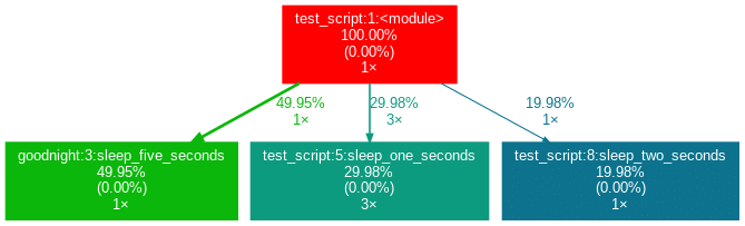
The script to be profiled always acts as a starting point and is the root of the tree. Each box is captioned with a function’s name, the overall percentage of time spent in the function, and its number of calls. The number in brackets represents the time spent in the function’s code, excluding time spent in other functions that are called in it.
In this case, all time is spent in the external module time‘s function sleep, which is why the number is 0.00%. Rarely a lot of time is spent in self-written functions, as the workload of a script usually quickly trickles down to very low-level functions of the Python implementation itself. Also, next to the arrows is the amount of time that one function passes to the other, along with the number of calls. The colors (RED-GREEN-BLUE, descending) and the thickness of the arrows indicate the relevance of different spots in the program.
Note that the percentages of the three functions above don’t add up to 100%. The reason behind is is that the graph is set up to only include self-written functions. In this case, the importing the time module caused the Python interpreter to spend 0.04% time in a function of the module importlib.
Evaluation with External Packages
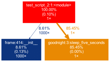
Consider a second example:
# test_script_2.py

import pandas as pd
from tests.goodnight import sleep_five_seconds

# some random madness
for i in range(1000):
   a_frame = pd.DataFrame([[1,2,3]])

sleep_five_seconds()
capture this in the graph, we can add the external package (pandas) with the -x flag. However, initializing a Pandas DataFrame is done within many pandas-internal functions. Frankly, I am personally not interested in the inner convolutions of pandas which is why I want the tree to not “sprout” too deep into the pandas mechanics. This can be accounted for by allowing only functions to show up if a minimal percentage of the runtime is spent in them.
Exactly this can be done using the -mflag. In combination, project_graph -m 8 -x pandas test_script_2.py yields the following:
Toy examples aside, let’s move on to something more serious. A real-life data-science project could look like this one:
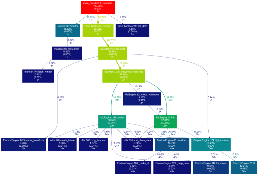
This time the tree is much bigger. It is actually even bigger than what you see in the illustration, as many more self-written functions are invoked. However, they are trimmed from the tree for clarity, as functions in which less than 0.5 % of the overall time is spent are filtered out (this is the default setting for the -m flag). Note that such a graph also really shines when searching for performance bottlenecks. One can see right away which functions carry most of the workload, when they are called, and how often they are called. This may prevent you from optimizing your program in the wrong spots while ignoring the elephant in the room.
How to Use Project Graphs
Installation
Within your project’s environment, do the following:
brew install graphviz

pip install git+https://github.com/fior-di-latte/project_graph.git
Usage
Within your project’s environment, change your current working directory to the project’s root (this is important!) and then enterfor standard usage:
project_graph myscript.pyIf your script includes an argparser, use:
project_graph "myscript.py <arg1> <arg2> (...)"If you want to see the entire graph, including all external packages, use:
project_graph -a myscript.pyIf you want to use a visibility threshold other than 1%, use:
project_graph -m <percent_value> myscript.pyFinally, if you want to include external packages into the graph, you can specify them as follows:
project_graph -x <package1> -x <package2> (...) myscript.pyConclusion & Caveats
This package has certain weaknesses, most of which can be addressed, e.g., by formatting the code into a function-based style, by trimming with the -m flag, or adding packages by using the -x flag. Generally, if something seems odd, the best first step is probably to use the -a flag to debug. Significant caveats are the following:
- It only works on Unix systems.
- It does not show a truthful graph when used with multiprocessing. The reason behind that is that cProfile is not compatible with multiprocessing. If multiprocessing is used, only the root process will be profiled, leading to false computation times in the graph. Switch to a non-parallel version of the target script.
- Profiling a script can lead to a considerable overhead computation-wise. It can make sense to scale down the work done in your script (i.e., decrease the amount of input data). If so, the time spent in the functions, of course, can be distorted massively if the functions don’t scale linearly.
- Nested functions will not show up in the graph. In particular, a decorator implicitly nests your function and will thus hide your function. That said, when using an external decorator, don’t forget to add the decorator’s package via the
-xflag (for example,project_graph -x numba myscript.py). - If your self-written function is exclusively called from an external package’s function, you must manually add the external package with the
-xflag. Otherwise, your function will not show up in the tree, as its parent is an external function and thus not considered.
Feel free to use the little package for your own project, be it for performance analysis, code introductions for new team members, or out of sheer curiosity. As for me, I find it very satisfying to see such a visualization of my projects. If you have trouble using it, don’t hesitate to hit me up on Github.
PS: If you’re looking for a similar package in R, check out Jakob’s post on flowcharts of functions.
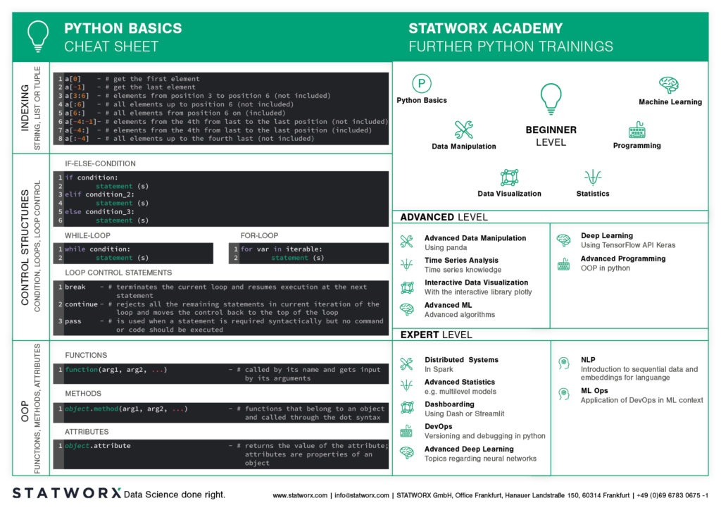
Do you want to learn Python? Or are you an R pro and you regularly miss the important functions and commands when working with Python? Or maybe you need a little reminder from time to time while coding? That’s exactly why cheatsheets were invented!
Cheatsheets help you in all these situations. Our first cheatsheet with Python basics is the start of a new blog series, where more cheatsheets will follow in our unique STATWORX style.
So you can be curious about our series of new Python cheatsheets that will cover basics as well as packages and workspaces relevant to Data Science.
Our cheatsheets are freely available for you to download, without registration or any other paywall.
Why have we created new cheatsheets?
As an experienced R user you will search endlessly for state-of-the-art Python cheatsheets similiar to those known from R Studio.
Sure, there are a lot of cheatsheets for every topic, but they differ greatly in design and content. As soon as we use several cheatsheets in different designs, we have to reorientate ourselves again and again and thus lose a lot of time in total. For us as data scientists it is important to have uniform cheatsheets where we can quickly find the desired function or command.
We want to counteract this annoying search for information. Therefore, we would like to regularly publish new cheatsheets in a design language on our blog in the future – and let you all participate in this work relief.
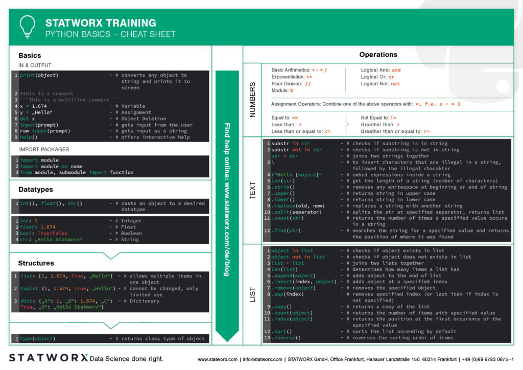
What does the first cheatsheet contain?
Our first cheatsheet in this series is aimed primarily at Python novices, R users who use Python less often, or peoples who are just starting to use it. It facilitates the introduction and overview in Python.
It makes it easier to get started and get an overview of Python. Basic syntax, data types, and how to use them are introduced, and basic control structures are introduced. This way, you can quickly access the content you learned in our STATWORX Academy, for example, or recall the basics for your next programming project.
What does the STATWORX Cheatsheet Episode 2 cover?
The next cheatsheet will cover the first step of a data scientist in a new project: Data Wrangling. Also, you can expect a cheatsheet for pandas about data loading, selection, manipulation, aggregation and merging. Happy coding!
In the , we discussed transfer learning and built a model for car model classification. In this blog post, we will discuss the problem of model deployment, using the TransferModel introduced in the first post as an example.
A model is of no use in actual practice if there is no simple way to interact with it. In other words: We need an API for our models. TensorFlow Serving has been developed to provide these functionalities for TensorFlow models. This blog post will show how a TensorFlow Serving server can be launched in a Docker container and how we can interact with the server using HTTP requests.
If you are new to Docker, we recommend working through Docker’s before reading this article. If you want to look at an example of deployment in Docker, we recommend reading this , in which he describes how an R-script can be run in Docker. We start by giving an overview of TensorFlow Serving.
Introduction to TensorFlow Serving
Let’s start by giving you an overview of TensorFlow Serving.
TensorFlow Serving is TensorFlow’s serving system, designed to enable the deployment of various models using a uniform API. Using the abstraction of Servables, which are basically objects clients use to perform computations, it is possible to serve multiple versions of deployed models. That enables, for example, that a new version of a model can be uploaded while the previous version is still available to clients. Looking at the bigger picture, so-called Managers are responsible for handling the life-cycle of Servables, which means loading, serving, and unloading them.
In this post, we will show how a single model version can be deployed. The code examples below show how a server can be started in a Docker container and how the Predict API can be used to interact with it. To read more about TensorFlow Serving, we refer to the .
Implementation
We will now discuss the following three steps required to deploy the model and to send requests.
- Save a model in correct format and folder structure using TensorFlow SavedModel
- Run a Serving server inside a Docker container
- Interact with the model using REST requests
Saving TensorFlow Models
If you didn’t read this series’ first post, here’s a brief summary of the most important points needed to understand the code below:
The TransferModel.model is a tf.keras.Model instance, so it can be saved using Model‘s built-in save method. Further, as the model was trained on web-scraped data, the class labels can change when re-scraping the data. We thus store the index-class mapping when storing the model in classes.pickle. TensorFlow Serving requires the model to be stored in the . When using tf.keras.Model.save, the path must be a folder name, else the model will be stored in another format (e.g., HDF5) which is not compatible with TensorFlow Serving. Below, folderpath contains the path of the folder we want to store all model relevant information in. The SavedModel is stored in folderpath/model and the class mapping is stored as folderpath/classes.pickle.
def save(self, folderpath: str):
    """
    Save the model using tf.keras.model.save

    Args:
        folderpath: (Full) Path to folder where model should be stored
    """

    # Make sure folderpath ends on slash, else fix
    if not folderpath.endswith("/"):
        folderpath += "/"

    if self.model is not None:
        os.mkdir(folderpath)
        model_path = folderpath + "model"
        # Save model to model dir
        self.model.save(filepath=model_path)
        # Save associated class mapping
        class_df = pd.DataFrame({'classes': self.classes})
        class_df.to_pickle(folderpath + "classes.pickle")
    else:
        raise AttributeError('Model does not exist')
Start TensorFlow Serving in Docker Container
Having saved the model to the disk, you now need to start the TensorFlow Serving server. Fortunately, there is an easy-to-use Docker container available. The first step is therefore pulling the TensorFlow Serving image from DockerHub. That can be done in the terminal using the command docker pull tensorflow/serving.
Then we can use the code below to start a TensorFlow Serving container. It runs the shell command for starting a container. The options set in the docker_run_cmd are the following:
- The serving image exposes port 8501 for the REST API, which we will use later to send requests. Thus we map the host port 8501 to the container’s 8501 port using
-p. - Next, we mount our model to the container using
-v. It is essential that the model is stored in a versioned folder (here MODEL_VERSION=1); else, the serving image will not find the model.model_path_guestthus must be of the form<path>/<model name>/MODEL_VERSION, whereMODEL_VERSIONis an integer. - Using
-e, we can set the environment variableMODEL_NAMEto our model’s name. - The
--name tf_servingoption is only needed to assign a specific name to our new docker container.
If we try to run this file twice in a row, the docker command will not be executed the second time, as a container with the name tf_serving already exists. To avoid this problem, we use docker_run_cmd_cond. Here, we first check if a container with this specific name already exists and is running. If it does, we leave it; if not, we check if an exited version of the container exists. If it does, it is deleted, and a new container is started; if not, a new one is created directly.
import os

MODEL_FOLDER = 'models'
MODEL_SAVED_NAME = 'resnet_unfreeze_all_filtered.tf'
MODEL_NAME = 'resnet_unfreeze_all_filtered'
MODEL_VERSION = '1'

# Define paths on host and guest system
model_path_host = os.path.join(os.getcwd(), MODEL_FOLDER, MODEL_SAVED_NAME, 'model')
model_path_guest = os.path.join('/models', MODEL_NAME, MODEL_VERSION)

# Container start command
docker_run_cmd = f'docker run ' \
                 f'-p 8501:8501 ' \
                 f'-v {model_path_host}:{model_path_guest} ' \
                 f'-e MODEL_NAME={MODEL_NAME} ' \
                 f'-d ' \
                 f'--name tf_serving ' \
                 f'tensorflow/serving'

# If container is not running, create a new instance and run it
docker_run_cmd_cond = f'if [ ! "$(docker ps -q -f name=tf_serving)" ]; then \n' \
                      f'   if [ "$(docker ps -aq -f status=exited -f name=tf_serving)" ]; then 														\n' \
                      f'   		docker rm tf_serving \n' \
                      f'   fi \n' \
                      f'   {docker_run_cmd} \n' \
                      f'fi'

# Start container
os.system(docker_run_cmd_cond)
Instead of mounting the model from our local disk using the -v flag in the docker command, we could also copy the model into the docker image, so the model could be served simply by running a container and specifying the port assignments. It is important to note that, in this case, the model needs to be saved using the folder structure folderpath/<model name>/1, as explained above. If this is not the case, TensorFlow Serving will not find the model. We will not go into further detail here. If you are interested in deploying your models in this way, we refer to on the TensorFlow website.
REST Request
Since the model is now served and ready to use, we need a way to interact with it. TensorFlow Serving provides two options to send requests to the server: and REST API, both exposed at different ports. In the following code example, we will use REST to query the model.
First, we load an image from the disk for which we want a prediction. This can be done using TensorFlow’s image module. Next, we convert the image to a numpy array using the img_to_array-method. The next and final step is crucial: since we preprocessed the training image before we trained our model (e.g., normalization), we need to apply the same transformation to the image we want to predict. The handypreprocess_input function makes sure that all necessary transformations are applied to our image.
from tensorflow.keras.preprocessing import image
from tensorflow.keras.applications.resnet_v2 import preprocess_input

# Load image
img = image.load_img(path, target_size=(224, 224))
img = image.img_to_array(img)

# Preprocess and reshape data
import json
import requests
# Send image as list to TF serving via json dump
request_url = 'http://localhost:8501/v1/models/resnet_unfreeze_all_filtered:predict'
request_body = json.dumps({"signature_name": "serving_default", "instances": img.tolist()})
request_headers = {"content-type": "application/json"}
json_response = requests.post(request_url, data=request_body, headers=request_headers)
response_body = json.loads(json_response.text)
predictions = response_body['predictions']
# Get label from prediction
y_hat_idx = np.argmax(predictions)
y_hat = classes[y_hat_idx]img = preprocess_input(img) img = img.reshape(-1, *img.shape)TensorFlow Serving’s RESTful API offers several endpoints. In general, the API accepts post requests following this structure:
POST http://host:port/<URI>:<VERB>

URI: /v1/models/${MODEL_NAME}[/versions/${MODEL_VERSION}]
VERB: classify|regress|predict
For our model, we can use the following URL for predictions:
The port number (here 8501) is the host’s port we specified above to map to the serving image’s port 8501. As mentioned above, 8501 is the serving container’s port exposed for the REST API. The model version is optional and will default to the latest version if omitted.
In python, the requests library can be used to send HTTP requests. As stated in the , the request body for the predict API must be a JSON object with the below-listed key-value-pairs:
signature_name– serving signature to use (for more information, see the )instances– model input in row format
The response body will also be a JSON object with a single key called predictions. Since we get for each row in the instances the probability for all 300 classes, we use np.argmax to return the most likely class. Alternatively, we could have used the higher-level classify API.
Conclusion
In this second blog article of the Car Model Classification series, we learned how to deploy a TensorFlow model for image recognition using TensorFlow Serving as a RestAPI, and how to run model queries with it.
To do so, we first saved the model using the SavedModel format. Next, we started the TensorFlow Serving server in a Docker container. Finally, we showed how to request predictions from the model using the API endpoints and a correct specified request body.
A major criticism of deep learning models of any kind is the lack of explainability of the predictions. In the third blog post, we will show how to explain model predictions using a method called Grad-CAM.
At STATWORX, we are very passionate about the field of deep learning. In this blog series, we want to illustrate how an end-to-end deep learning project can be implemented. We use TensorFlow 2.x library for the implementation. The topics of the series include:
- Transfer learning for computer vision.
- Model deployment via TensorFlow Serving.
- Interpretability of deep learning models via Grad-CAM.
- Integrating the model into a Dash dashboard.
In the first part, we will show how you can use transfer learning to tackle car image classification. We start by giving a brief overview of transfer learning and the ResNet and then go into the implementation details. The code presented can be found in this github repository.
Introduction: Transfer Learning & ResNet
What is Transfer Learning?
In traditional (machine) learning, we develop a model and train it on new data for every new task at hand. Transfer learning differs from this approach in that knowledge is transferred from one task to another. It is a useful approach when one is faced with the problem of too little available training data. Models that are pretrained for a similar problem can be used as a starting point for training new models. The pretrained models are referred to as base models.
In our example, a deep learning model trained on the ImageNet dataset can be used as the starting point for building a car model classifier. The main idea behind transfer learning for deep learning models is that the first layers of a network are used to extract important high-level features, which remain similar for the kind of data treated. The final layers (also known as the head) of the original network are replaced by a custom head suitable for the problem at hand. The weights in the head are initialized randomly, and the resulting network can be trained for the specific task.
There are various ways in which the base model can be treated during training. In the first step, its weights can be fixed. If the learning progress suggests the model not being flexible enough, certain layers or the entire base model can be “unfrozen” and thus made trainable. A further important aspect to note is that the input must be of the same dimensionality as the data on which the model was trained on – if the first layers of the base model are not modified.

Next, we will briefly introduce the ResNet, a popular and powerful CNN architecture for image data. Then, we will show how we used transfer learning with ResNet to do car model classification.
What is ResNet?
Training deep neural networks can quickly become challenging due to the so-called vanishing gradient problem. But what are vanishing gradients? Neural networks are commonly trained using back-propagation. This algorithm leverages the chain rule of calculus to derive gradients at deeper layers of the network by multiplying gradients from earlier layers. Since gradients get repeatedly multiplied in deep networks, they can quickly approach infinitesimally small values during back-propagation.
ResNet is a CNN network that solves the vanishing gradient problem using so-called residual blocks (you find a good explanation of why they are called ‘residual’ here). The unmodified input is passed on to the next layer in the residual block by adding it to a layer’s output (see right figure). This modification makes sure that a better information flow from the input to the deeper layers is possible. The entire ResNet architecture is depicted in the right network in the left figure below. It is plotted alongside a plain CNN and the VGG-19 network, another standard CNN architecture.
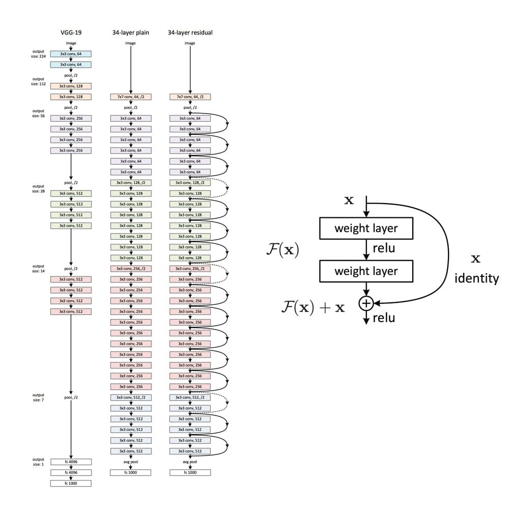
ResNet has proved to be a powerful network architecture for image classification problems. For example, an ensemble of ResNets with 152 layers won the ILSVRC 2015 image classification contest. Pretrained ResNet models of different sizes are available in the tensorflow.keras.application module, namely ResNet50, ResNet101, ResNet152 and their corresponding second versions (ResNet50V2, …). The number following the model name denotes the number of layers the networks have. The available weights are pretrained on the ImageNet dataset. The models were trained on large computing clusters using hardware accelerators for significant time periods. Transfer learning thus enables us to leverage these training results using the obtained weights as a starting point.
Classifying Car Models
As an illustrative example of how transfer learning can be applied, we treat the problem of classifying the car model given an image of the car. We will start by describing the dataset set we used and how we can filter out unwanted examples in the dataset. Next, we will go over how a data pipeline can be setup using tensorflow.data. In the second section, we will talk you through the model implementation and point out what aspects to be particularly careful about during training and prediction.
Data Preparation
We used the dataset described in this github repo, where you can also download the entire dataset. The author built a datascraper to scrape all car images from the car connection website. He explains that many images are from the interior of the cars. As they are not wanted in the dataset, they are filtered out based on pixel color. The dataset contains 64’467 jpg images, where the file names contain information on the car’s make, model, build year, etc. For a more detailed insight on the dataset, we recommend you consult the original github repo. Three sample images are shown below.

While checking through the data, we observed that the dataset still contained many unwanted images, e.g., pictures of wing mirrors, door handles, GPS panels, or lights. Examples of unwanted images can be seen below.

Thus, it is beneficial to additionally prefilter the data to clean out more of the unwanted images.
Filtering Unwanted Images Out of the Dataset
There are multiple possible approaches to filter non-car images out of the dataset:
- Use a pretrained model
- Train another model to classify car/no-car
- Train a generative network on a car dataset and use the discriminator part of the network
We decided to pursue the first approach since it is the most direct one and outstanding pretrained models are easily available. If you want to follow the second or third approach, you could, e.g., use this dataset to train the model. The referred dataset only contains images of cars but is significantly smaller than the dataset we used.
We chose the ResNet50V2 in the tensorflow.keras.applications module with the pretrained “imagenet” weights. In a first step, we must figure out the indices and classnames of the imagenet labels corresponding to car images.
# Class labels in imagenet corresponding to cars
CAR_IDX = [656, 627, 817, 511, 468, 751, 705, 757, 717, 734, 654, 675, 864, 609, 436]

CAR_CLASSES = ['minivan', 'limousine', 'sports_car', 'convertible', 'cab', 'racer', 'passenger_car', 'recreational_vehicle', 'pickup', 'police_van', 'minibus', 'moving_van', 'tow_truck', 'jeep', 'landrover', 'beach_wagon']
Next, the pretrained ResNet50V2 model is loaded.
from tensorflow.keras.applications import ResNet50V2

model = ResNet50V2(weights='imagenet')
We can then use this model to make predictions for images. The images fed to the prediction method must be scaled identically to the images used for training. The different ResNet models are trained on different input scales. It is thus essential to apply the correct image preprocessing. The module keras.application.resnet_v2 contains the method preprocess_input, which should be used when using a ResNetV2 network. This method expects the image arrays to be of type float and have values in [0, 255]. Using the appropriately preprocessed input, we can then use the built-in predict method to obtain predictions given an image stored at filename:
from tensorflow.keras.applications.resnet_v2 import preprocess_input

image = tf.io.read_file(filename)
image = tf.image.decode_jpeg(image)
image = tf.cast(image, tf.float32)
image = tf.image.resize_with_crop_or_pad(image, target_height=224, target_width=224)
image = preprocess_input(image)
predictions = model.predict(image)
There are various ideas of how the obtained predictions can be used for car detection.
- Is one of the
CAR_CLASSESamong the top k predictions? - Is the accumulated probability of the
CAR_CLASSESin the predictions greater than some defined threshold? - Specific treatment of unwanted images (e.g., detect and filter out wheels)
We show the code for comparing the accumulated probability mass over the CAR_CLASSES.
def is_car_acc_prob(predictions, thresh=THRESH, car_idx=CAR_IDX):
    """
    Determine if car on image by accumulating probabilities of car prediction and comparing to threshold

    Args:
        predictions: (?, 1000) matrix of probability predictions resulting from ResNet with imagenet weights
        thresh: threshold accumulative probability over which an image is considered a car
        car_idx: indices corresponding to cars

    Returns:
        np.array of booleans describing if car or not
    """
    predictions = np.array(predictions, dtype=float)
    car_probs = predictions[:, car_idx]
    car_probs_acc = car_probs.sum(axis=1)
    return car_probs_acc > thresh
The higher the threshold is set, the stricter the filtering procedure is. A value for the threshold that provides good results is THRESH = 0.1. This ensures we do not lose too many true car images. The choice of an appropriate threshold remains subjective, so do as you feel.
The Colab notebook that uses the function is_car_acc_prob to filter the dataset is available in the github repository.
While tuning the prefiltering procedure, we observed the following:
- Many of the car images with light backgrounds were classified as “beach wagons”. We thus decided to also consider the “beach wagon” class in imagenet as one of the
CAR_CLASSES. - Images showing the front of a car are often assigned a high probability of “grille”, which is the grating at the front of a car used for cooling. This assignment is correct but leads the procedure shown above to not consider certain car images as cars since we did not include “grille” in the
CAR_CLASSES. This problem results in the trade-off of either leaving many close-up images of car grilles in the dataset or filtering out several car images. We opted for the second approach since it yields a cleaner car dataset.
After prefiltering the images using the suggested procedure, 53’738 of 64’467 initially remain in the dataset.
Overview of the Final Datasets
The prefiltered dataset contains images from 323 car models. We decided to reduce our attention to the top 300 most frequent classes in the dataset. That makes sense since some of the least frequent classes have less than ten representatives and can thus not be reasonably split into a train, validation, and test set. Reducing the dataset to images in the top 300 classes leaves us with a dataset containing 53’536 labeled images. The class occurrences are distributed as follows:

The number of images per class (car model) ranges from 24 to slightly below 500. We can see that the dataset is very imbalanced. It is essential to keep this in mind when training and evaluating the model.
Building Data Pipelines with tf.data
Even after prefiltering and reducing to the top 300 classes, we still have numerous images left. This poses a potential problem since we can not simply load all images into the memory of our GPU at once. To tackle this problem, we will use tf.data.
tf.data and especially the tf.data.Dataset API allows creating elegant and, at the same time, very efficient input pipelines. The API contains many general methods which can be applied to load and transform potentially large datasets. tf.data.Dataset is especifically useful when training models on GPU(s). It allows for data loading from the HDD, applies transformation on-the-fly, and creates batches that are than sent to the GPU. And this is all done in a way such as the GPU never has to wait for new data.
The following functions create a tf.data.Dataset instance for our particular problem:
def construct_ds(input_files: list,
                 batch_size: int,
                 classes: list,
                 label_type: str,
                 input_size: tuple = (212, 320),
                 prefetch_size: int = 10,
                 shuffle_size: int = 32,
                 shuffle: bool = True,
                 augment: bool = False):
    """
    Function to construct a tf.data.Dataset set from list of files

    Args:
        input_files: list of files
        batch_size: number of observations in batch
        classes: list with all class labels
        input_size: size of images (output size)
        prefetch_size: buffer size (number of batches to prefetch)
        shuffle_size: shuffle size (size of buffer to shuffle from)
        shuffle: boolean specifying whether to shuffle dataset
        augment: boolean if image augmentation should be applied
        label_type: 'make' or 'model'

    Returns:
        buffered and prefetched tf.data.Dataset object with (image, label) tuple
    """
    # Create tf.data.Dataset from list of files
    ds = tf.data.Dataset.from_tensor_slices(input_files)

    # Shuffle files
    if shuffle:
        ds = ds.shuffle(buffer_size=shuffle_size)

    # Load image/labels
    ds = ds.map(lambda x: parse_file(x, classes=classes, input_size=input_size,                                                                                                                                        label_type=label_type))

    # Image augmentation
    if augment and tf.random.uniform((), minval=0, maxval=1, dtype=tf.dtypes.float32, seed=None, name=None) < 0.7:
        ds = ds.map(image_augment)

    # Batch and prefetch data
    ds = ds.batch(batch_size=batch_size)
    ds = ds.prefetch(buffer_size=prefetch_size)

    return ds
We will now describe the methods in the tf.data we used:
from_tensor_slices()is one of the available methods for the creation of a dataset. The created dataset contains slices of the given tensor, in this case, the filenames.- Next, the
shuffle()method considersbuffer_sizeelements one at a time and shuffles these items in isolation from the rest of the dataset. If shuffling of the complete dataset is required,buffer_sizemust be larger than the bumber of entries in the dataset. Shuffling is only performed ifshuffle=True. map()allows to apply arbitrary functions to the dataset. We created a functionparse_file()that can be found in the github repo. It is responsible for reading and resizing the images, inferring the labels from the file name and encoding the labels using a one-hot encoder. If the augment flag is set, the data augmentation procedure is activated. Augmentation is only applied in 70% of the cases since it is beneficial to also train the model on non-modified images. The augmentation techniques used inimage_augmentare flipping, brightness, and contrast adjustments.- Finally, the
batch()method is used to group the dataset into batches ofbatch_sizeelements and theprefetch()method enables preparing later elements while the current element is being processed and thus improves performance. If used after a call tobatch(),prefetch_sizebatches are prefetched.
Model Fine Tuning
Having defined our input pipeline, we now turn towards the model training part. Below you can see the code that can be used to instantiate a model based on the pretrained ResNet, which is available in tf.keras.applications:
from tensorflow.keras.applications import ResNet50V2
from tensorflow.keras import Model
from tensorflow.keras.layers import Dense, GlobalAveragePooling2D


class TransferModel:

    def __init__(self, shape: tuple, classes: list):
        """
        Class for transfer learning from ResNet

        Args:
            shape: Input shape as tuple (height, width, channels)
            classes: List of class labels
        """
        self.shape = shape
        self.classes = classes
        self.history = None
        self.model = None

        # Use pre-trained ResNet model
        self.base_model = ResNet50V2(include_top=False,
                                     input_shape=self.shape,
                                     weights='imagenet')

        # Allow parameter updates for all layers
        self.base_model.trainable = True

        # Add a new pooling layer on the original output
        add_to_base = self.base_model.output
        add_to_base = GlobalAveragePooling2D(data_format='channels_last', name='head_gap')(add_to_base)

        # Add new output layer as head
        new_output = Dense(len(self.classes), activation='softmax', name='head_pred')(add_to_base)

        # Define model
        self.model = Model(self.base_model.input, new_output)
A few more details on the code above:
- We first create an instance of class
tf.keras.applications.ResNet50V2. Withinclude_top=Falsewe tell the pretrained model to leave out the original head of the model (in this case designed for the classification of 1000 classes on ImageNet). base_model.trainable = Truemakes all layers trainable.- Using
tf.kerasfunctional API, we then stack a new pooling layer on top of the last convolution block of the original ResNet model. This is a necessary intermediate step before feeding the output to the final classification layer. - The final classification layer is then defined using
tf.keras.layers.Dense. We define the number of neurons to be equal to the number of desired classes. And the softmax activation function makes sure that the output is a pseudo probability in the range of(0,1].
The full version of TransferModel (see github) also contains the option to replace the base model with a VGG16 network, another standard CNN for image classification. In addition, it also allows to unfreeze only specific layers, meaning we can make the corresponding parameters trainable while leaving the others fixed. As a default, we have made all parameters trainable here.
After we defined the model, we need to configure it for training. This can be done using tf.keras.Model‘s compile()-method:
def compile(self, **kwargs):
      """
    Compile method
    """
    self.model.compile(**kwargs)
We then pass the following keyword arguments to our method:
loss = "categorical_crossentropy"for multi-class classification,optimizer = Adam(0.0001)for using the Adam optimizer fromtf.keras.optimizerswith a relatively small learning rate (more on the learning rate below), andmetrics = ["categorical_accuracy"]for training and validation monitoring.
Next, we will look at the training procedure. Therefore we define a train-method for our TransferModel-class introduced above:
from tensorflow.keras.callbacks import EarlyStopping

def train(self,
          ds_train: tf.data.Dataset,
          epochs: int,
          ds_valid: tf.data.Dataset = None,
          class_weights: np.array = None):
    """
    Trains model in ds_train with for epochs rounds

    Args:
        ds_train: training data as tf.data.Dataset
        epochs: number of epochs to train
        ds_valid: optional validation data as tf.data.Dataset
        class_weights: optional class weights to treat unbalanced classes

    Returns
        Training history from self.history
    """

    # Define early stopping as callback
    early_stopping = EarlyStopping(monitor='val_loss',
                                   min_delta=0,
                                   patience=12,
                                   restore_best_weights=True)

    callbacks = [early_stopping]

    # Fitting
    self.history = self.model.fit(ds_train,
                                  epochs=epochs,
                                  validation_data=ds_valid,
                                  callbacks=callbacks,
                                  class_weight=class_weights)

    return self.history
As our model is an instance of tensorflow.keras.Model, we can train it using the fit method. To prevent overfitting, early stopping is used by passing it to the fit method as a callback function. The patience parameter can be tuned to specify how soon early stopping should apply. The parameter stands for the number of epochs after which, if no decrease of the validation loss is registered, the training will be interrupted. Further, class weights can be passed to the fit method. Class weights allow treating unbalanced data by assigning the different classes different weights, thus allowing to increase the impact of classes with fewer training examples.
We can describe the training process using a pretrained model as follows: As the weights in the head are initialized randomly, and the weights of the base model are pretrained, the training composes of training the head from scratch and fine-tuning the pretrained model’s weights. It is recommended to use a small learning rate (e.g. 1e-4) since choosing the learning rate too large can destroy the near-optimal pretrained weights of the base model.
The training procedure can be sped up by first training for a few epochs without the base model being trainable. The purpose of these initial epochs is to adapt the heads’ weights to the problem. This speeds up the training since when training only the head, much fewer parameters are trainable and thus updated for every batch. The resulting model weights can then be used as the starting point to train the entire model, with the base model being trainable. For the car classification problem that we are considering here, applying this two-stage training did not achieve notable performance enhancement.
Model Performance Evaluation/Prediction
When using the tf.data.Dataset API, one must pay attention to the nature of the methods used. The following method in our TransferModel class can be used as a prediction method.
def predict(self, ds_new: tf.data.Dataset, proba: bool = True):
    """
    Predict class probs or labels on ds_new
    Labels are obtained by taking the most likely class given the predicted probs

    Args:
        ds_new: New data as tf.data.Dataset
        proba: Boolean if probabilities should be returned

    Returns:
        class labels or probabilities
    """

    p = self.model.predict(ds_new)

    if proba:
        return p
    else:
        return [np.argmax(x) for x in p]
It is essential that the dataset ds_new is not shuffled, or else the predictions obtained will be misaligned with the images obtained when iterating over the dataset a second time. This is the case since the flag reshuffle_each_iteration is true by default in the shuffle method’s implementation. A further effect of shuffling is that multiple calls to the take method will not return the same data. This is important when you want to check out predictions, e.g., for only one batch. A simple example where this can be seen is:
# Use construct_ds method from above to create a shuffled dataset
ds = construct_ds(..., shuffle=True)

# Take 1 batch (e.g. 32 images) of dataset: This returns a new dataset
ds_batch = ds.take(1)

# Predict labels for one batch
predictions = model.predict(ds_batch)

# Predict labels again: The result will not be the same as predictions above due to shuffling
predictions_2 = model.predict(ds_batch)
A function to plot images annotated with the corresponding predictions could look as follows:
def show_batch_with_pred(model, ds, classes, rescale=True, size=(10, 10), title=None):
      for image, label in ds.take(1):
        image_array = image.numpy()
        label_array = label.numpy()
        batch_size = image_array.shape[0]
        pred = model.predict(image, proba=False)
        for idx in range(batch_size):
            label = classes[np.argmax(label_array[idx])]
            ax = plt.subplot(np.ceil(batch_size / 4), 4, idx + 1)
            if rescale:
                plt.imshow(image_array[idx] / 255)
            else:
                plt.imshow(image_array[idx])
            plt.title("label: " + label + "\n"
                      + "prediction: " + classes[pred[idx]], fontsize=10)
            plt.axis('off')
The show_batch_with_pred method works for shuffled datasets as well, since image and label correspond to the same call to the take method.
Evaluating model perfomance can be done using keras.Model's evaluate method.
How Accurate Is Our Final Model?
The model achieves slightly above 70% categorical accuracy for the task of predicting the car model for images from 300 model classes. To better understand the model’s predictions, it is helpful to observe the confusion matrix. Below, you can see the heatmap of the model’s predictions on the validation dataset.

We restricted the heatmap to clip the confusion matrix’s entries to [0, 5], as allowing a further span did not significantly highlight any off-diagonal region. As can be seen from the heat map, one class is assigned to examples of almost all classes. That can be seen from the dark red vertical line two-thirds to the right in the figure above. Other than the class mentioned before, there are no evident biases in the predictions. We want to stress here that the categorical accuracy is generally not sufficient for a satisfactory assessment of the model’s performance, particularly in the case of imbalanced classes.
Conclusion and Next Steps
In this blog post, we have applied transfer learning using the ResNet50V2 to classify the car model from images of cars. Our model achieves 70% categorical accuracy over 300 classes.
We found unfreezing the entire base model and using a small learning rate to achieve the best results. Now, having developed a cool car classification model is great, but how can we use our model in a productive setting? Of course, we could build our custom model API using Flask or FastAPI…
But might there even be an easier, standardized way? In the second article of our series, “Deploying TensorFlow Models in Docker using TensorFlow Serving“, we discuss how this model can be deployed using TensorFlow Serving.
Management Summary
OCR (Optical Character Recognition) is a major challenge for many companies. The OCR market is comprised of various open source and commercial providers. A well-known open source tool for OCR is Tesseract, which is provided by Google. Tesseract is currently available in version 4, which performs OCR extraction using recurrent neural networks. However, the OCR performance of Tesseract is still volatile and depends on various factors. A particular challenge is the application of Tesseract to documents that are composed of different structures, e.g. texts, tables and images. Invoices, for example, are such a type of document, and OCR tools from all vendors continue to underperform on this document type.
This article demonstrates how fine-tuning the Tesseract OCR engine on a small sample of data can already significantly improve OCR performance on invoice documents. The presented process is not only applicable to invoices but to any type of document.
A use case is defined aimed at a correct extraction of all text (words and numbers) from one fictional yet realistic German invoice. It’s fictively assumed that the extracted information is destined for downstream accounting purposes. Therefore, a correct extraction of numbers and the Euro-symbol is considered to be critical.
The OCR performance of two Tesseract models for the German language is compared: the standard (non-fine-tuned) model and its fine-tuned variant. The standard model is downloaded from the Tesseract OCR GitHub repository. The fine-tuned model is created using the steps outlined in this article. A second German invoice similar to the first one is used for fine-tuning. Both the standard model and fine-tuned model are evaluated on the first German invoice to ensure a fair comparison.
The OCR performance of the standard model on numbers is poor. Certain numbers are falsely recognized as other numbers. This is especially true for numbers that look similar like the number 1 and 7. The Euro-symbol is falsely recognized in 50% of the cases, making the result unsuitable for any downstream accounting application.
The fine-tuned model shows a similar OCR performance for German words. However, the OCR performance on numbers improves significantly. All numbers and every Euro-symbol is extracted correctly.
It is concluded that fine-tuning can yield a large improvement for a minimal amount of effort and training data. This fact makes Tesseract OCR with its open-source licensing an attractive solution compared to propriety OCR software. Final recommendations are offered for fine-tuning Tesseract LTM models given a real use case for which more training data is available.
Introduction
Tesseract 4 with its LSTM engine works reasonably well out-of-the-box for plain text pages.
There are however certain challenging scenarios for which an off-the-shelf model performs poorly. Examples include texts written in exotic type fonts, images with backgrounds and text in tables. Luckily, Tesseract provides a way to fine-tune the LSTM engine to improve its OCR performance on a specific use case.
In this article the OCR (Optical Character Recognition) performance of an off-the-shelf Tesseract LSTM model is benchmarked on a German invoice. Next this this model is fine-tuned on a second German invoice. The OCR performance of both models is compared, and further improvements are suggested.
Why OCR on invoices remains challenging
Even though OCR is considered to be a solved problem, extracting a large corpus of text without any mistakes remains challenging. This is especially true for OCR on invoice documents which, compared to a book-type text, face three additional problems:
- colored backgrounds and table structures pose a challenge for page segmentation
- invoices typically contain rare characters such as the EUR or USD sign
- numbers can’t be verified against a language dictionary
In addition, the margin for error is small: for accounting applications an exact extraction of numeric data is paramount for all subsequent process steps.
The first problem can generally be resolved by selecting a suitable page segmentation mode of the fourteen that are provided by Tesseract. The latter two problems can be resolved by fine-tuning the LSTM engine on examples of similar invoices.
Use case objective and data
Two similar example invoices are considered in the article. The first invoice shown in Figure 1 will be used to evaluate the OCR performance of both the standard and the fine-tuned Tesseract model. Special attention is devoted to the correct extraction of numbers for accounting purposes. The second invoice shown in Figure 2 will be used as training data to fine-tune Tesseract.
Invoices are mostly written in a very readable type font like “Arial”. To illustrate the benefits of fine-tuning, the initial OCR problem is made more challenging by considering invoices written in the font “Impact”. This is a font for which Tesseract struggles to resolve certain characters.
It will be shown that after fine-tuning on a very small amount of data, Tesseract will yield very satisfactory results in spite of this challenging font.
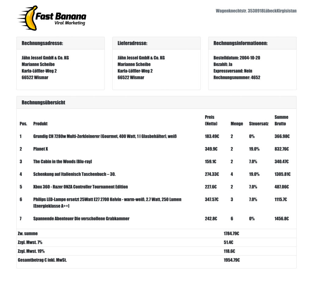
Figure 1: Evaluation invoice on which both the standard and fine-tuned Tesseract models will be evaluated
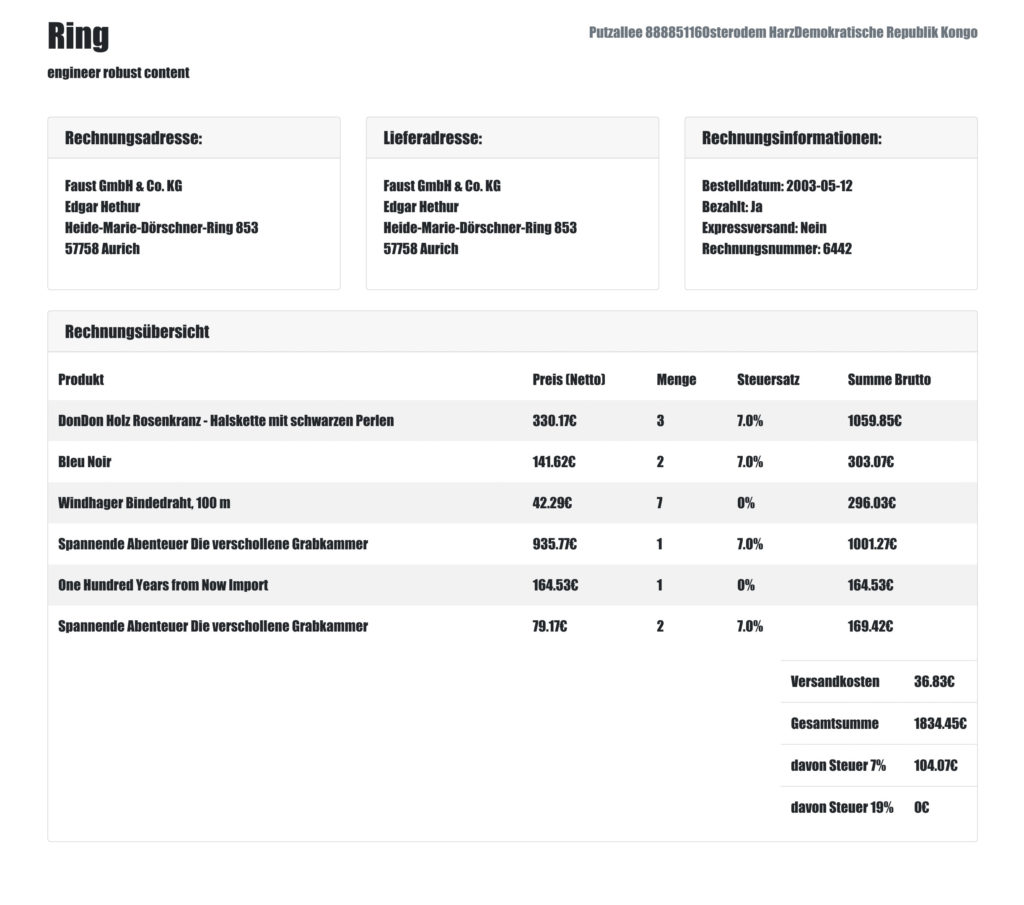
Figure 2: Training invoice on which the Tesseract OCR LSTM model will be fine-tuned
Using the Tesseract 4.1 Docker container
The set up for fine-tuning the Tesseract LSTM engine currently only works on Linux and can be a bit tricky. Therefore, a Docker container with pre-installed Tesseract 4.1, along with the compiled training tools and scripts, is provided with this article.
Pull the container image from Docker Hub and run the container’s shell to replicate the commands in this article:
docker pull statworx/blog-tesseract
docker run -it --name tesseract_container statworx/blog-tesseract /bin/bash
General improvements of OCR Performance
There are three ways in which Tesseract’s OCR performance can be improved before resorting to fine-tuning the LSTM engine.
1. Image preprocessing
Invoice images may have a skewed orientation if they weren’t properly aligned on the scanner. Rotated images should be deskewed to improve Tesseract’s line segmentation performance.
In addition, scanning may introduce image noise which should be removed by a denoising algorithm. Note that by default Tesseract performs thresholding using Otsu’s algorithm to binarize grayscale images into black and white pixels.
A thorough treatment of image preprocessing is beyond the scope of this article and is not necessary to obtain satisfactory results in the given use case. The Tesseract documentation provides a convenient overview.
2. Page segmentation
During page segmentation Tesseract attempts to identify rectangular regions of text.
Only these regions are selected for OCR in the next step. It’s therefore critical to capture all regions with text lest information be lost.
Tesseract allows to choose from 14 different page segmentation methods that can be viewed by using the following the command:
tesseract --help-psmThe default segmentation method expects a page of text similar to a book page. However, this mode fails to identify all text regions on an invoice because of its additional tabular structure. A better segmentation method is given by option 4: Assume a single column of text of variable sizes.
To illustrate the importance of a suitable page segmentation method, consider the result of using the default method “Fully automatic page segmentation, but no OSD” in Figure 3:
Figure 3: Page segmentation using the default method fails to determine all text regions
Note that the text „Rechnungsinformationen:”, “Pos.” and “Produkt” were not segmented. In Figure 4 a more suitable method results in a perfect page segmentation.
3. Use of dictionaries, word lists and patterns for text
The LSTM models used by Tesseract were trained on large amounts of text in one specific language. This command shows the languages that are currently available for Tesseract:
tesseract --list-langs Additional language models can be obtained by downloading the corresponding language.tessdata and placing it in the tessdata folder of the local Tesseract installation. The Tesseract repository on GitHub provides three variants of language models: normal, fast and best. Only the fast and best variants are suitable for fine-tuning. As their name implies, they are the fastest and most accurate variants of models respectively. Other models have also been trained for specific use cases like exclusively recognizing digits and punctuation and are listed in the references.
As the language of the invoices in this use case are German, the Docker image belonging to this article comes with the deu.tessdata model.
For a chosen language, Tesseract’s word list can be further expanded or limited to certain words or even characters. This subject lies outside the scope of this article as it’s not necessary to obtain satisfactory results in this use case.
Setup for the fine-tuning process
Three file types must be created for fine-tuning:
1. tiff files
Tagged Image File Format or TIFF is an uncompressed image file format (as opposed to JPG or PNG which are compressed file formats). TIFF files can be obtained from PNG or JPG formats by a conversion tool. Although Tesseract can work with PNG and JPG images, the TIFF format is recommended.
2. box files
To train the LSTM model Tesseract relies on so called box files with the “.box” extension. A box file contains the recognized text along with the coordinates of the bounding box in which the text is situated. Box files contain six columns representing symbol, left, bottom, right, top and page.
P 157 2566 1465 2609 0
r 157 2566 1465 2609 0
o 157 2566 1465 2609 0
d 157 2566 1465 2609 0
u 157 2566 1465 2609 0
k 157 2566 1465 2609 0
t 157 2566 1465 2609 0
  157 2566 1465 2609 0
P 157 2566 1465 2609 0
r 157 2566 1465 2609 0
e 157 2566 1465 2609 0
i 157 2566 1465 2609 0
s 157 2566 1465 2609 0
  157 2566 1465 2609 0
( 157 2566 1465 2609 0
N 157 2566 1465 2609 0
e 157 2566 1465 2609 0
t 157 2566 1465 2609 0
t 157 2566 1465 2609 0
o 157 2566 1465 2609 0
) 157 2566 1465 2609 0
  157 2566 1465 2609 0
Each individual character is situated on a separate line in the box file. The LSTM model accepts either the coordinates of individual characters or a whole text line. In the example box file above the text “Produkt Preis (Netto)” is located on the same line. All characters have the same coordinates, namely the coordinates of the bounding box around that text line. Using line-level coordinates is considerably easier and will be provided by default when the box file is generated with the following command:
cd /home/fine_tune/train
tesseract train_invoice.tiff train_invoice --psm 4 -l best/deu lstmbox
The first argument is the image file, the second the box file name. The language parameter -l instructs Tesseract to use the German model for OCR. The parameter –psm instructs Tesseract to use page segmentation method number four.
Unavoidably, the generated box files OCR will contain errors in the symbol column. Each symbol in the training box file must therefore be verified by hand. This is a tedious process given that the box file of the train invoice contains nearly a thousand lines (one for each character in the invoice). To simplify the correction, the Docker container provides a Python script that draws the bounding boxes along with the OCR text on the original invoice image for easier comparison. The result is shown in Figure 4. The Docker container already contains the corrected box files indicated by the suffix “_correct”.
Figure 4: Extracted text using the standard German model “deu”
3. lstmf files
During fine-tuning Tesseract extracts text from the tiff file using OCR and verifies its prediction using the coordinates and the symbol in the box file. Tesseract does not rely on the tiff and box file directly, but expects an lstmf file constructed from both previous files. Note that in order to create the lstmf file the tiff and box files must have the same name, for example train_invoice.tiff and train_invoice.box.
The following command generates an lstmf file for the train invoice:
cd /home/fine_tune/train
tesseract train_invoice.tiff train_invoice lstm.train
All lstmf files destined for training must be specified by their relative path in a text file called deu.training_files.txt. In this use case only one lstmf file will be used for training so the deu.training_files.txt contains just one line: eval/train_invoice_correct.lstmf.
It’s recommended to create an lstfm file for the eval invoice as well. This way the model performance can be evaluated during model training.
cd /home/fine_tune/eval
tesseract eval_invoice_correct.tiff eval_invoice_correct lstm.train
Evaluating the standard LSTM model
OCR predictions from the standard German model “deu” will serve as a benchmark. An accurate overview of the standard German model’s OCR performance can be obtained by generating a box file for the eval invoice and visualizing the OCR text using the Python script mentioned earlier. This Python script that generates the file ‘eval_invoice_ocr deu.tiff’ is located under /home/fine_tune/src/draw_box_file_data.py in the Docker. It expects the path to a tiff file, the corresponding box file and a name for the output tiff file. The OCR text extracted by the standard German model is saved as eval/eval_invoice_ocr_deu.tiff and shown in Figure 1.
At first glance the text extracted by OCR looks good. The model correctly extracts German characters such as ä, ö ü and ß. In fact, there are only three occasions where words contain errors:
| OCR | Truth |
| Jessel GmbH 8 Co | Jessel GmbH & Co |
| 11 Glasbehälter | 1l Glasbehälter |
| Zeki64@hloch.com | Zeki64@bloch.com |
The German model performs well on common German words but has difficulties with singular symbols such as “&”and “l” and words such as “bloch” that are not present in the model’s word list.
Prices and numbers in general are a different story. Here the errors are numerous.
| OCR | Truth |
| 159,16 | 159,1€ |
| 1% | 7% |
| 1305.816 | 1305.81€ |
| 227.66 | 227.6€ |
| 341.51 | 347.57€ |
| 1115.16 | 1115.7€ |
| 242.86 | 242.8€ |
| 1456.86 | 1456.8€ |
| 51.46 | 54.1€ |
| 1954.719€ | 1954.79€ |
Note that the standard German model failed to extract the Euro-symbol € in 9 of 18 occurrences. This represents an error rate of 50%.
Fine-tuning the standard LSTM model
The LSTM model will now be fine-tuned on the training invoice shown in Figure 2. Next the OCR performance will be evaluated on the evaluation invoice shown in Figure 1 that was used for benchmarking the standard German model.
To fine-tune the LSTM model it must first be extracted from the deu.traineddata. The following command extracts the LSTM model from the standard German into the directory lstm_model:
cd /home/fine_tune
combine_tessdata -e tesseract/tessdata/best/deu.traineddata lstm_model/deu.lstm
Now all necessary files are obtained for fine-tuning. The files are also present in the Docker container:
- The training files train_invoice_correct.lstmf and deu.training_files.txt in the train directory.
- The evaluation files eval_invoice_correct.lstmf and deu.training_files.txt in the eval directory.
- The extracted LSTM model deu.lstm in the lstm_model directory.
The Docker container contains the script src/fine_tune.sh that launches the fine-tuning process. Its contents are:
/usr/local/bin/lstmtraining \
  --model_output output/fine_tuned \
  --continue_from lstm_model/deu.lstm \
  --traineddata tesseract/tessdata/best/deu.traineddata \
  --train_listfile train/deu.training_files.txt \
  --eval_listfile eval/deu.training_files.txt \
  --max_iterations 400
This command fine-tunes the extracted deu.lstm model on the train_invoice.lstmf file specified in train/deu.training_files.txt. Fine-tuning the LSTM model requires language-specific information that is contained in the deu.tessdata folder. The eval_invoice.lstmf file specified in eval/deu.training_files.txt will be used to compute OCR performance metrics during training. Fine-tuning will stop after 400 iterations. The total training duration takes less than two minutes.
The following command runs the script and logs the output to a file:
cd /home/fine_tune
sh src/fine_tune.sh > output/fine_tune.log 2>&1
The contents of the log file after training are shown below:
src/fine_tune.log
Loaded file lstm_model/deu.lstm, unpacking...
Warning: LSTMTrainer deserialized an LSTMRecognizer!
Continuing from lstm_model/deu.lstm
Loaded 20/20 lines (1-20) of document train/train_invoice_correct.lstmf
Loaded 24/24 lines (1-24) of document eval/eval_invoice_correct.lstmf

2 Percent improvement time=69, best error was 100 @ 0
At iteration 69/100/100, Mean rms=1.249%, delta=2.886%, char train=8.17%, word train=22.249%, skip ratio=0%, New best char error = 8.17 Transitioned to stage 1 wrote best model:output/deu_fine_tuned8.17_69.checkpoint wrote checkpoint.
-----
2 Percent improvement time=62, best error was 8.17 @ 69
At iteration 131/200/200, Mean rms=1.008%, delta=2.033%, char train=5.887%, word train=20.832%, skip ratio=0%, New best char error = 5.887 wrote best model:output/deu_fine_tuned5.887_131.checkpoint wrote checkpoint.
-----
2 Percent improvement time=112, best error was 8.17 @ 69
At iteration 181/300/300, Mean rms=0.88%, delta=1.599%, char train=4.647%, word train=17.388%, skip ratio=0%, New best char error = 4.647 wrote best model:output/deu_fine_tuned4.647_181.checkpoint wrote checkpoint.
-----
2 Percent improvement time=159, best error was 8.17 @ 69
At iteration 228/400/400, Mean rms=0.822%, delta=1.416%, char train=4.144%, word train=16.126%, skip ratio=0%, New best char error = 4.144 wrote best model:output/deu_fine_tuned4.144_228.checkpoint wrote checkpoint.
-----
Finished! Error rate = 4.144
During training Tesseract saves a model checkpoint after every iteration. The performance of the model at this checkpoint is tested on the evaluation data and compared against the current best score. If the score improves, i.e. the character error decreases, a labeled copy of the checkpoint is saved. The first number of the checkpoint’s label represents the character error and the second number the training iteration.
The last step that remains is to re-assemble the fine-tuned LSTM model so that once again a “traineddata” model is obtained. Assuming the checkpoint at the 139th iteration is desired, the following command converts a chosen checkpoint “deu_fine_tuned4.647_181.checkpoint” into a fully functional Tesseract model “deu_fine_tuned.traineddata”:
cd /home/fine_tune
/usr/local/bin/lstmtraining \
  --stop_training \
  --continue_from output/deu_fine_tuned4.647_181.checkpoint \
  --traineddata tesseract/tessdata/best/deu.traineddata \
  --model_output tesseract/tessdata/best/deu_fine_tuned.traineddata
This model must be copied into the tessdata of the local Tesseract installation to make it available to Tesseract. This has already been done in the Docker container.
Verify that the fine-tuned model is available in Tesseract:
tesseract --list-langsEvaluating the fine-tuned LSTM model
The fine-tuned model will be evaluated analogously to the standard model: a box file of the evaluation invoice is created, and the OCR text is displayed on the evaluation invoice image using the Python script.
The command to generate the box files must be modified to use the fine-tuned model “deu_fine_tuned” instead of the standard model “deu”:
cd /home/fine_tune/eval
tesseract eval_invoice.tiff eval_invoice --psm 4 -l best/deu_fine_tuned lstmbox
The OCR text extracted by the fine-tuned model is shown in Figure 5 below.
Figure 5: OCR using the fine-tuned German model “deu_fine_tuned”
As with the standard German model, the performance on words remains good but not perfect. To improve the performance on rare words the model’s word list could be expanded to include specific jargon.
| OCR | Truth |
| Jessel GmbH 8 Co | Jessel GmbH & Co |
| 1! Glasbehälte | 1l Glasbehälter |
| Zeki64@hloch.com | Zeki64@bloch.com |
More importantly, the OCR performance on numbers has improved significantly:The fine-tuned model extracted all numbers and every occurrence of the € sign correctly.
| OCR | Truth |
| 159,1€ | 159,1€ |
| 7% | 7% |
| 1305.81€ | 1305.81€ |
| 227.6€ | 227.6€ |
| 347.57€ | 347.57€ |
| 1115.7€ | 1115.7€ |
| 242.8€ | 242.8€ |
| 1456.8€ | 1456.8€ |
| 54.1€ | 54.1€ |
| 1954.79€ | 1954.79€ |
Conclusion and further improvements
In this article it was demonstrated that the performance on a difficult problem such as OCR on German invoices written in the challenging font “impact” is greatly improved by fine-tuning on just one example invoice. The ability to fine-tune on a specific use case combined with its open-source licensing makes Tesseract OCR version 4 with its LSTM engine an attractive solution to tackle challenging OCR problems.
It might be tempting to run the fine-tuning for more iterations to improve the accuracy even further. In this use case the number of iterations was deliberately limited because only one training invoice was used. More iterations increase the risk of overfitting the LSTM model on certain symbols which increases the error rate of other symbols. In practice though, it’s desirable to increase the number of iterations on the condition that sufficient training data is provided. Nevertheless, finding the optimal number of iterations is more an art than a science. The final OCR performance should always be verified on a different yet representative set of evaluation data.
References
Tesseract training: https://tesseract-ocr.github.io/tessdoc/TrainingTesseract-4.00.html
Image processing overview: https://tesseract-ocr.github.io/tessdoc/ImproveQuality#image-processing
Otsu thresholding: https://opencv-python-tutroals.readthedocs.io/en/latest/py_tutorials/py_imgproc/py_thresholding/py_thresholding.html
Tesseract digits comma model: https://github.com/Shreeshrii/tessdata_shreetest
Introduction
When working on data science projects in R, exporting internal R objects as files on your hard drive is often necessary to facilitate collaboration. Here at STATWORX, we regularly export R objects (such as outputs of a machine learning model) as .RDS files and put them on our internal file server. Our co-workers can then pick them up for further usage down the line of the data science workflow (such as visualizing them in a dashboard together with inputs from other colleagues).
Over the last couple of months, I came to work a lot with RDS files and noticed a crucial shortcoming: The base R saveRDS function does not allow for any kind of archiving of existing same-named files on your hard drive. In this blog post, I will explain why this might be very useful by introducing the basics of serialization first and then showcasing my proposed solution: A wrapper function around the existing base R serialization framework.
Be wary of silent file replacements!
In base R, you can easily export any object from the environment to an RDS file with:
saveRDS(object = my_object, file = "path/to/dir/my_object.RDS")However, including such a line somewhere in your script can carry unintended consequences: When calling saveRDS multiple times with identical file names, R silently overwrites existing, identically named .RDS files in the specified directory. If the object you are exporting is not what you expect it to be — for example due to some bug in newly edited code — your working copy of the RDS file is simply overwritten in-place. Needless to say, this can prove undesirable.
If you are familiar with this pitfall, you probably used to forestall such potentially troublesome side effects by commenting out the respective lines, then carefully checking each time whether the R object looked fine, then executing the line manually. But even when there is nothing wrong with the R object you seek to export, it can make sense to retain an archived copy of previous RDS files: Think of a dataset you run through a data prep script, and then you get an update of the raw data, or you decide to change something in the data prep (like removing a variable). You may wish to archive an existing copy in such cases, especially with complex data prep pipelines with long execution time.
Don’t get tangled up in manual renaming
You could manually move or rename the existing file each time you plan to create a new one, but that’s tedious, error-prone, and does not allow for unattended execution and scalability. For this reason, I set out to write a carefully designed wrapper function around the existing saveRDS call, which is pretty straightforward: As a first step, it checks if the file you attempt to save already exists in the specified location. If it does, the existing file is renamed/archived (with customizable options), and the “updated” file will be saved under the originally specified name.
This approach has the crucial advantage that the existing code that depends on the file name remaining identical (such as readRDS calls in other scripts) will continue to work with the latest version without any needs for adjustment! No more saving your objects as “models_2020-07-12.RDS”, then combing through the other scripts to replace the file name, only to repeat this process the next day. At the same time, an archived copy of the — otherwise overwritten — file will be kept.
What are RDS files anyways?
Before I walk you through my proposed solution, let’s first examine the basics of serialization, the underlying process behind high-level functions like saveRDS.
Simply speaking, serialization is the “process of converting an object into a stream of bytes so that it can be transferred over a network or stored in a persistent storage.” Stack Overflow: What is serialization?
There is also a low-level R interface, serialize, which you can use to explore (un-)serialization first-hand: Simply fire up R and run something like serialize(object = c(1, 2, 3), connection = NULL). This call serializes the specified vector and prints the output right to the console. The result is an odd-looking raw vector, with each byte separately represented as a pair of hex digits. Now let’s see what happens if we revert this process:
s <- serialize(object = c(1, 2, 3), connection = NULL)
print(s)
# >  [1] 58 0a 00 00 00 03 00 03 06 00 00 03 05 00 00 00 00 05 55 54 46 2d 38 00 00 00 0e 00
# > [29] 00 00 03 3f f0 00 00 00 00 00 00 40 00 00 00 00 00 00 00 40 08 00 00 00 00 00 00

unserialize(s)
# > 1 2 3
The length of this raw vector increases rapidly with the complexity of the stored information: For instance, serializing the famous, although not too large, iris dataset results in a raw vector consisting of 5959 pairs of hex digits!
Besides the already mentioned saveRDS function, there is also the more generic save function. The former saves a single R object to a file. It allows us to restore the object from that file (with the counterpart readRDS), possibly under a different variable name: That is, you can assign the contents of a call to readRDS to another variable. By contrast, save allows for saving multiple R objects, but when reading back in (with load), they are simply restored in the environment under the object names they were saved with. (That’s also what happens automatically when you answer “Yes” to the notorious question of whether to “save the workspace image to ~/.RData” when quitting RStudio.)
Creating the archives
Obviously, it’s great to have the possibility to save internal R objects to a file and then be able to re-import them in a clean session or on a different machine. This is especially true for the results of long and computationally heavy operations such as fitting machine learning models. But as we learned earlier, one wrong keystroke can potentially erase that one precious 3-hour-fit fine-tuned XGBoost model you ran and carefully saved to an RDS file yesterday.

Digging into the wrapper
So, how did I go about fixing this? Let’s take a look at the code. First, I define the arguments and their defaults: The object and file arguments are taken directly from the wrapped function, the remaining arguments allow the user to customize the archiving process: Append the archive file name with either the date the original file was archived or last modified, add an additional timestamp (not just the calendar date), or save the file to a dedicated archive directory. For more details, please check the documentation here. I also include the ellipsis ... for additional arguments to be passed down to saveRDS. Additionally, I do some basic input handling (not included here).
save_rds_archive <- function(object,
                             file = "",
                             archive = TRUE,
                             last_modified = FALSE,
                             with_time = FALSE,
                             archive_dir_path = NULL,
                             ...) {
The main body of the function is basically a series of if/else statements. I first check if the archive argument (which controls whether the file should be archived in the first place) is set to TRUE, and then if the file we are trying to save already exists (note that “file” here actually refers to the whole file path). If it does, I call the internal helper function create_archived_file, which eliminates redundancy and allows for concise code.
if (archive) {

    # check if file exists
    if (file.exists(file)) {

      archived_file <- create_archived_file(file = file,
                                            last_modified = last_modified,
                                            with_time = with_time)
Composing the new file name
In this function, I create the new name for the file which is to be archived, depending on user input: If last_modified is set, then the mtime of the file is accessed. Otherwise, the current system date/time (= the date of archiving) is taken instead. Then the spaces and special characters are replaced with underscores, and, depending on the value of the with_time argument, the actual time information (not just the calendar date) is kept or not.
To make it easier to identify directly from the file name what exactly (date of archiving vs. date of modification) the indicated date/time refers to, I also add appropriate information to the file name. Then I save the file extension for easier replacement (note that “.RDS”, “.Rds”, and “.rds” are all valid file extensions for RDS files). Lastly, I replace the current file extension with a concatenated string containing the type info, the new date/time suffix, and the original file extension. Note here that I add a “$” sign to the regex which is to be matched by gsub to only match the end of the string: If I did not do that and the file name would be something like “my_RDS.RDS”, then both matches would be replaced.
# create_archived_file.R

create_archived_file <- function(file, last_modified, with_time) {

  # create main suffix depending on type
  suffix_main <- ifelse(last_modified,
                        as.character(file.info(file)$mtime),
                        as.character(Sys.time()))

  if (with_time) {

    # create clean date-time suffix
    suffix <- gsub(pattern = " ", replacement = "_", x = suffix_main)
    suffix <- gsub(pattern = ":", replacement = "-", x = suffix)

    # add "at" between date and time
    suffix <- paste0(substr(suffix, 1, 10), "_at_", substr(suffix, 12, 19))

  } else {

    # create date suffix
    suffix <- substr(suffix_main, 1, 10)

  }

  # create info to paste depending on type
  type_info <- ifelse(last_modified,
                      "_MODIFIED_on_",
                      "_ARCHIVED_on_")

  # get file extension (could be any of "RDS", "Rds", "rds", etc.)
  ext <- paste0(".", tools::file_ext(file))

  # replace extension with suffix
  archived_file <- gsub(pattern = paste0(ext, "$"),
                        replacement = paste0(type_info,
                                             suffix,
                                             ext),
                        x = file)

  return(archived_file)

}
Archiving the archives?
By way of example, with last_modified = FALSE and with_time = TRUE, this function would turn the character file name “models.RDS” into “models_ARCHIVED_on_2020-07-12_at_11-31-43.RDS”. However, this is just a character vector for now — the file itself is not renamed yet. For this, we need to call the base R file.rename function, which provides a direct interface to your machine’s file system. I first check, however, whether a file with the same name as the newly created archived file string already exists: This could well be the case if one appends only the date (with_time = FALSE) and calls this function several times per day (or potentially on the same file if last_modified = TRUE).
Somehow, we are back to the old problem in this case. However, I decided that it was not a good idea to archive files that are themselves archived versions of another file since this would lead to too much confusion (and potentially too much disk space being occupied). Therefore, only the most recent archived version will be kept. (Note that if you still want to keep multiple archived versions of a single file, you can set with_time = TRUE. This will append a timestamp to the archived file name up to the second, virtually eliminating the possibility of duplicated file names.) A warning is issued, and then the already existing archived file will be overwritten with the current archived version.
The last puzzle piece: Renaming the original file
To do this, I call the file.rename function, renaming the “file” originally passed by the user call to the string returned by the helper function. The file.rename function always returns a boolean indicating if the operation succeeded, which I save to a variable temp to inspect later. Under some circumstances, the renaming process may fail, for instance due to missing permissions or OS-specific restrictions. We did set up a CI pipeline with GitHub Actions and continuously test our code on Windows, Linux, and MacOS machines with different versions of R. So far, we didn’t run into any problems. Still, it’s better to provide in-built checks.
It’s an error! Or is it?
The problem here is that, when renaming the file on disk failed, file.rename raises merely a warning, not an error. Since any causes of these warnings most likely originate from the local file system, there is no sense in continuing the function if the renaming failed. That’s why I wrapped it into a tryCatch call that captures the warning message and passes it to the stop call, which then terminates the function with the appropriate message.
Just to be on the safe side, I check the value of the temp variable, which should be TRUE if the renaming succeeded, and also check if the archived version of the file (that is, the result of our renaming operation) exists. If both of these conditions hold, I simply call saveRDS with the original specifications (now that our existing copy has been renamed, nothing will be overwritten if we save the new file with the original name), passing along further arguments with ....
        if (file.exists(archived_file)) {
          warning("Archived copy already exists - will overwrite!")
        }

        # rename existing file with the new name
        # save return value of the file.rename function
        # (returns TRUE if successful) and wrap in tryCatch
        temp <- tryCatch({file.rename(from = file,
                                      to = archived_file)
        },
        warning = function(e) {
          stop(e)
        })

      }

      # check return value and if archived file exists
      if (temp & file.exists(archived_file)) {
        # then save new file under specified name
        saveRDS(object = object, file = file, ...)
      }

    }
These code snippets represent the cornerstones of my function. I also skipped some portions of the source code for reasons of brevity, chiefly the creation of the “archive directory” (if one is specified) and the process of copying the archived file into it. Please refer to our GitHub for the complete source code of the main and the helper function.
Finally, to illustrate, let’s see what this looks like in action:
x <- 5
y <- 10
z <- 20

## save to RDS
saveRDS(x, "temp.RDS")
saveRDS(y, "temp.RDS")

## "temp.RDS" is silently overwritten with y
## previous version is lost
readRDS("temp.RDS")
#> [1] 10

save_rds_archive(z, "temp.RDS")
## current version is updated
readRDS("temp.RDS")
#> [1] 20

## previous version is archived
readRDS("temp_ARCHIVED_on_2020-07-12.RDS")
#> [1] 10
Great, how can I get this?
The function save_rds_archive is now included in the newly refactored helfRlein package (now available in version 1.0.0!) which you can install directly from GitHub:
# install.packages("devtools")
devtools::install_github("STATWORX/helfRlein")
Feel free to check out additional documentation and the source code there. If you have any inputs or feedback on how the function could be improved, please do not hesitate to contact me or raise an issue on our GitHub.
Conclusion
That’s it! No more manually renaming your precious RDS files — with this function in place, you can automate this tedious task and easily keep a comprehensive archive of previous versions. You will be able to take another look at that one model you ran last week (and then discarded again) in the blink of an eye. I hope you enjoyed reading my post — maybe the function will come in handy for you someday!
Because You Are Interested In Data Science, You Are Interested In This Blog Post
If you love streaming movies and tv series online as much as we do here at STATWORX, you’ve probably stumbled upon recommendations like “Customers who viewed this item also viewed…” or “Because you have seen …, you like …”. Amazon, Netflix, HBO, Disney+, etc. all recommend their products and movies based on your previous user behavior – But how do these companies know what their customers like? The answer is collaborative filtering.
In this blog post, I will first explain how collaborative filtering works. Secondly, I’m going to show you how to develop your own small movie recommender with the R package recommenderlab and provide it in a shiny application.
Different Approaches
There are several approaches to give a recommendation. In the user-based collaborative filtering (UBCF), the users are in the focus of the recommendation system. For a new proposal, the similarities between new and existing users are first calculated. Afterward, either the n most similar users or all users with a similarity above a specified threshold are consulted. The average ratings of the products are formed via these users and, if necessary, weighed according to their similarity. Then, the x highest rated products are displayed to the new user as a suggestion.
For the item-based collaborative filtering IBCF, however, the focus is on the products. For every two products, the similarity between them is calculated in terms of their ratings. For each product, the k most similar products are identified, and for each user, the products that best match their previous purchases are suggested.
Those and other collaborative filtering methods are implemented in the recommenderlab package:
- ALS_realRatingMatrix: Recommender for explicit ratings based on latent factors, calculated by alternating least squares algorithm.
- ALS_implicit_realRatingMatrix: Recommender for implicit data based on latent factors, calculated by alternating least squares algorithm.
- IBCF_realRatingMatrix: Recommender based on item-based collaborative filtering.
- LIBMF_realRatingMatrix: Matrix factorization with LIBMF via package recosystem.
- POPULAR_realRatingMatrix: Recommender based on item popularity.
- RANDOM_realRatingMatrix: Produce random recommendations (real ratings).
- RERECOMMEND_realRatingMatrix: Re-recommends highly-rated items (real ratings).
- SVD_realRatingMatrix: Recommender based on SVD approximation with column-mean imputation.
- SVDF_realRatingMatrix: Recommender based on Funk SVD with gradient descend.
- UBCF_realRatingMatrix: Recommender based on user-based collaborative filtering.
Developing your own Movie Recommender
Dataset
To create our recommender, we use the data from movielens. These are film ratings from 0.5 (= bad) to 5 (= good) for over 9000 films from more than 600 users. The movieId is a unique mapping variable to merge the different datasets.
head(movie_data) movieId title genres
1 1 Toy Story (1995) Adventure|Animation|Children|Comedy|Fantasy
2 2 Jumanji (1995) Adventure|Children|Fantasy
3 3 Grumpier Old Men (1995) Comedy|Romance
4 4 Waiting to Exhale (1995) Comedy|Drama|Romance
5 5 Father of the Bride Part II (1995) Comedy
6 6 Heat (1995) Action|Crime|Thrillerhead(ratings_data) userId movieId rating timestamp
1 1 1 4 964982703
2 1 3 4 964981247
3 1 6 4 964982224
4 1 47 5 964983815
5 1 50 5 964982931
6 1 70 3 964982400To better understand the film ratings better, we display the number of different ranks and the average rating per film. We see that in most cases, there is no evaluation by a user. Furthermore, the average ratings contain a lot of “smooth” ranks. These are movies that only have individual ratings, and therefore, the average score is determined by individual users.
# ranting_vector
0         0.5    1      1.5    2      2.5   3      3.5    4       4.5   5
5830804   1370   2811   1791   7551   5550  20047  13136  26818   8551  13211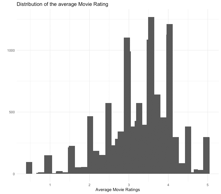
In order not to let individual users influence the movie ratings too much, the movies are reduced to those that have at least 50 ratings.
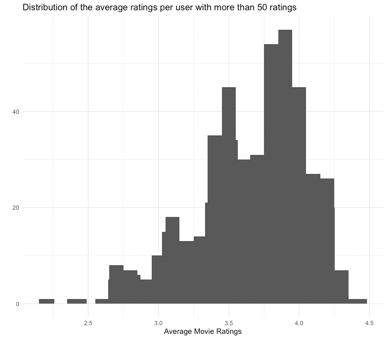
##    Min. 1st Qu.  Median    Mean 3rd Qu.    Max.
##   2.208   3.444   3.748   3.665   3.944   4.429
Under the assumption that the ratings of users who regularly give their opinion are more precise, we also only consider users who have given at least 50 ratings. For the films filtered above, we receive the following average ratings per user:
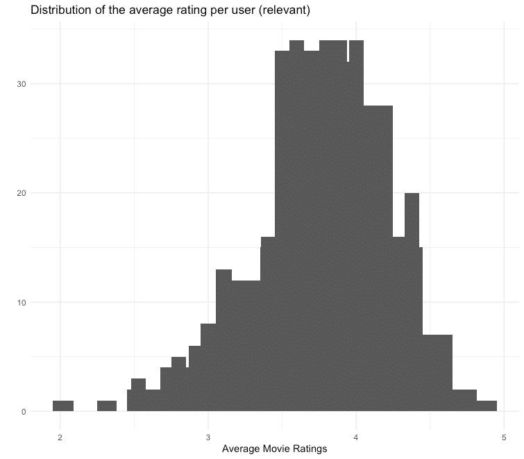
You can see that the distribution of the average ratings is left-skewed, which means that many users tend to give rather good ratings. To compensate for this skewness, we normalize the data.
ratings_movies_norm <- normalize(ratings_movies)Model Training and Evaluation
To train our recommender and subsequently evaluate it, we carry out a 10-fold cross-validation. Also, we train both an IBCF and a UBCF recommender, which in turn calculate the similarity measure via cosine similarity and Pearson correlation. A random recommendation is used as a benchmark. To evaluate how many recommendations can be given, different numbers are tested via the vector n_recommendations.
eval_sets <- evaluationScheme(data = ratings_movies_norm,
                              method = "cross-validation",
                              k = 10,
                              given = 5,
                              goodRating = 0)

models_to_evaluate <- list(
  `IBCF Cosinus` = list(name = "IBCF",
                        param = list(method = "cosine")),
  `IBCF Pearson` = list(name = "IBCF",
                        param = list(method = "pearson")),
  `UBCF Cosinus` = list(name = "UBCF",
                        param = list(method = "cosine")),
  `UBCF Pearson` = list(name = "UBCF",
                        param = list(method = "pearson")),
  `Zufälliger Vorschlag` = list(name = "RANDOM", param=NULL)
)

n_recommendations <- c(1, 5, seq(10, 100, 10))

list_results <- evaluate(x = eval_sets,
                         method = models_to_evaluate,
                         n = n_recommendations)
We then have the results displayed graphically for analysis.
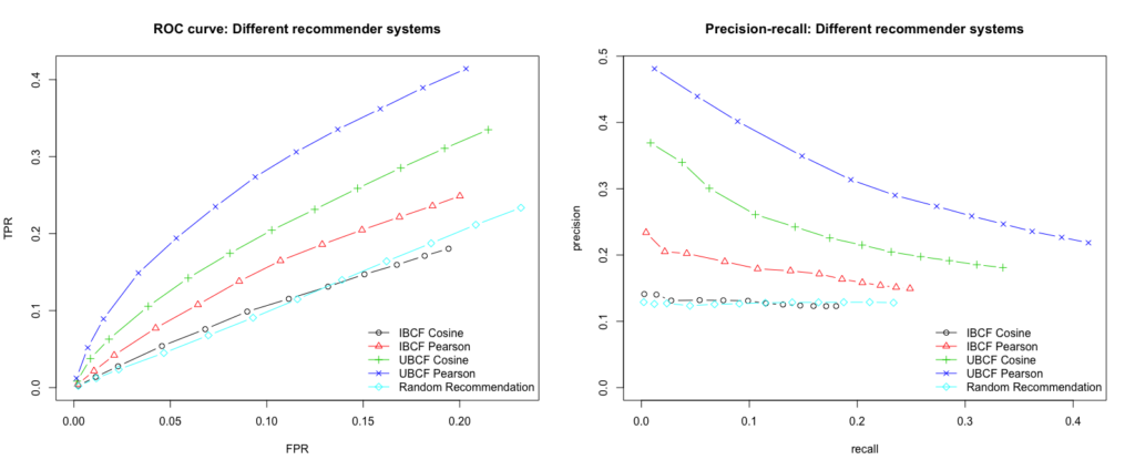
We see that the best performing model is built by using UBCF and the Pearson correlation as a similarity measure. The model consistently achieves the highest true positive rate for the various false-positive rates and thus delivers the most relevant recommendations. Furthermore, we want to maximize the recall, which is also guaranteed at every level by the UBCF Pearson model. Since the n most similar users (parameter nn) are used to calculate the recommendations, we will examine the results of the model for different numbers of users.
vector_nn <- c(5, 10, 20, 30, 40)

models_to_evaluate <- lapply(vector_nn, function(nn){
  list(name = "UBCF",
       param = list(method = "pearson", nn = vector_nn))
})
names(models_to_evaluate) <- paste0("UBCF mit ", vector_nn, "Nutzern")
list_results <- evaluate(x = eval_sets,
                         method = models_to_evaluate,
                         n = n_recommendations)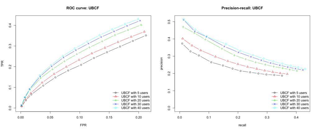
Conclusion
Our user based collaborative filtering model with the Pearson correlation as a similarity measure and 40 users as a recommendation delivers the best results. To test the model by yourself and get movie suggestions for your own flavor, I created a small Shiny App.
However, there is no guarantee that the suggested movies really meet the individual taste. Not only is the underlying data set relatively small and can still be distorted by user ratings, but the tech giants also use other data such as age, gender, user behavior, etc. for their models.
But what I can say is: Data Scientists who read this blog post also read the other blog posts by STATWORX.
Shiny-App
Here you can find the Shiny App. To get your own movie recommendation, select up to 10 movies from the dropdown list, rate them on a scale from 0 (= bad) to 5 (= good) and press the run button. Please note that the app is located on a free account of shinyapps.io. This makes it available for 25 hours per month. If the 25 hours are used and therefore the app is this month no longer available, you will find the code here to run it on your local RStudio.