Be Safe!
In the age of open-source software projects, attacks on vulnerable software are ever present. Python is the most popular language for Data Science and Engineering and is thus increasingly becoming a target for attacks through malicious libraries. Additionally, public facing applications can be exploited by attacking vulnerabilities in the source code.
For this reason it’s crucial that your code does not contain any CVEs (common vulnerabilities and exposures) or uses other libraries that might be malicious. This is especially true if it’s public facing software, e.g. a web application. At statworx we look for ways to increase the quality of our code by using automated scanning tools. Hence, we’ll discuss the value of two code and package scanners for Python.
Automatic screening
There are numerous tools for scanning code and its dependencies, here I will provide an overview of the most popular tools designed with Python in mind. Such tools fall into one of two categories:
- Static Application Security Testing (SAST): look for weaknesses in code and vulnerable packages
- Dynamic Application Security Testing (DAST): look for vulnerabilities that occur at runtime
In what follows I will compare bandit and safety using a small streamlit application I’ve developed. Both tools fall into the category of SAST, since they don’t need the application to run in order to perform their checks. Dynamic application testing is more involved and may be the subject of a future post.
The application
For the sake of context, here’s a brief description of the application: it was designed to visualize the convergence (or lack thereof) in the sampling distributions of random variables drawn from different theoretical probability distributions. Users can choose the distribution (e.g. Log-Normal), set the maximum number of samples and pick different sampling statistics (e.g. mean, standard deviation, etc.).
Bandit
Bandit is an open-source python code scanner that checks for vulnerabilities in code and only in your code. It decomposes the code into its abstract syntax tree and runs plugins against it to check for known weaknesses. Among other tests it performs checks on plain SQL code which could provide an opening for SQL injections, passwords stored in code and hints about common openings for attacks such as use of the pickle library. Bandit is designed for use with CI/CD and throws an exit status of 1 whenever it encounters any issues, thus terminating the pipeline. A report is generated, which includes information about the number of issues separated by confidence and severity according to three levels: low, medium, and high. In this case, bandit finds no obvious security flaws in our code.
Run started:2022-06-10 07:07:25.344619

Test results:
        No issues identified.

Code scanned:
        Total lines of code: 0
        Total lines skipped (#nosec): 0

Run metrics:
        Total issues (by severity):
                Undefined: 0
                Low: 0
                Medium: 0
                High: 0
        Total issues (by confidence):
                Undefined: 0
                Low: 0
                Medium: 0
                High: 0
Files skipped (0):
All the more reason to carefully configure Bandit to use in your project. Sometimes it may raise a flag even though you already know that this would not be a problem at runtime. If, for example, you have a series of unit tests that use pytest and run as part of your CI/CD pipeline Bandit will normally throw an error, since this code uses the assert statement, which is not recommended for code that does not run without the -O flag.
To avoid this behaviour you could:
- run scans against all files but exclude the test using the command line interface
- create a
yamlconfiguration file to exclude the test
Here’s an example:
# bandit_cfg.yml
skips: ["B101"] # skips the assert check
Then we can run bandit as follows: bandit -c bandit_yml.cfg /path/to/python/files and the unnecessary warnings will not crop up.
Safety
Developed by the team at pyup.io, this package scanner runs against a curated database which consists of manually reviewed records based on publicly available CVEs and changelogs. The package is available for Python >= 3.5 and can be installed for free. By default it uses Safety DB which is freely accessible. Pyup.io also offers paid access to a more frequently updated database.
Running safety check --full-report -r requirements.txt on the package root directory gives us the following output (truncated the sake of readability):
+==============================================================================+
|                                                                              |
|                               /$$$$$$            /$$                         |
|                              /$$__  $$          | $$                         |
|           /$$$$$$$  /$$$$$$ | $$  \__//$$$$$$  /$$$$$$   /$$   /$$           |
|          /$$_____/ |____  $$| $$$$   /$$__  $$|_  $$_/  | $$  | $$           |
|         |  $$$$$$   /$$$$$$$| $$_/  | $$$$$$$$  | $$    | $$  | $$           |
|          \____  $$ /$$__  $$| $$    | $$_____/  | $$ /$$| $$  | $$           |
|          /$$$$$$$/|  $$$$$$$| $$    |  $$$$$$$  |  $$$$/|  $$$$$$$           |
|         |_______/  \_______/|__/     \_______/   \___/   \____  $$           |
|                                                          /$$  | $$           |
|                                                         |  $$$$$$/           |
|  by pyup.io                                              \______/            |
|                                                                              |
+==============================================================================+
| REPORT                                                                       |
| checked 110 packages, using free DB (updated once a month)                   |
+============================+===========+==========================+==========+
| package                    | installed | affected                 | ID       |
+============================+===========+==========================+==========+
| urllib3                    | 1.26.4    | <1.26.5                  | 43975    |
+==============================================================================+
| Urllib3 1.26.5 includes a fix for CVE-2021-33503: An issue was discovered in |
| urllib3 before 1.26.5. When provided with a URL containing many @ characters |
| in the authority component, the authority regular expression exhibits        |
| catastrophic backtracking, causing a denial of service if a URL were passed  |
| as a parameter or redirected to via an HTTP redirect.                        |
| https://github.com/advisories/GHSA-q2q7-5pp4-w6pg                            |
+==============================================================================+
The report includes the number of packages that were checked, the type of database used for reference and information on each vulnerability that was found. In this example an older version of the package urllib3 is affected by a vulnerability which technically could be used by an to perform a denial-of-service attack.
Integration into your workflow
Both bandit and safety are available as GitHub Actions. The stable release of safety also provides integrations for TravisCI and GitLab CI/CD.
Of course, you can always manually install both packages from PyPI on your runner if no ready-made integration like a GitHub action is available. Since both programs can be used from the command line, you could also integrate them into a pre-commit hook locally if using them on your CI/CD platform is not an option.
The CI/CD pipeline for the application above was built with GitHub Actions. After installing the application’s required packages, it runs bandit first and then safety to scan all packages. With all the packages updated, the vulnerability scans pass and the docker image is built.
| Package check | Code Check |
|---|---|
 |
 |
Conclusion
I would strongly recommend using both bandit and safety in your CI/CD pipeline, as they provide security checks for your code and your dependencies. For modern applications manually reviewing every single package your application depends on is simply not feasible, not to mention all of the dependencies these packages have! Thus, automated scanning is inevitable if you want to have some level of awareness about how unsafe your code is.
While bandit scans your code for known exploits, it does not check any of the libraries used in your project. For this, you need safety, as it informs you about known security flaws in the libraries your application depends on. While neither frameworks are completely foolproof, it’s still better to be notified about some CVEs than none at all. This way, you’ll be able to either fix your vulnerable code or upgrade a vulnerable package dependency to a more secure version.
Keeping your code safe and your dependencies trustworthy can ward off potentially devastating attacks on your application.
Introduction
The more complex any given data science project in Python gets, the harder it usually becomes to keep track of how all modules interact with each other. Undoubtedly, when working in a team on a bigger project, as is often the case here at STATWORX, the codebase can soon grow to an extent where the complexity may seem daunting. In a typical scenario, each team member works in their “corner” of the project, leaving each one merely with firm local knowledge of the project’s code but possibly only a vague idea of the overall project architecture. Ideally, however, everyone involved in the project should have a good global overview of the project. By that, I don’t mean that one has to know how each function works internally but rather to know the responsibility of the main modules and how they are interconnected.
A visual helper for learning about the global structure can be a call graph. A call graph is a directed graph that displays which function calls which. It is created from the data of a Python profiler such as cProfile.
Since such a graph proved helpful in a project I’m working on, I created a package called project_graph, which builds such a call graph for any provided python script. The package creates a profile of the given script via cProfile, converts it into a filtered dot graph via gprof2dot, and finally exports it as a .png file.
Why Are Project Graphs Useful?
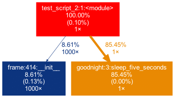
As a small first example, consider this simple module.
# test_script.py

import time
from tests.goodnight import sleep_five_seconds

def sleep_one_seconds():
    time.sleep(1)

def sleep_two_seconds():
    time.sleep(2)

for i in range(3):
    sleep_one_seconds()

sleep_two_seconds()

sleep_five_seconds()
After installation (see below), by writing project_graph test_script.py into the command line, the following png-file is placed next to the script:
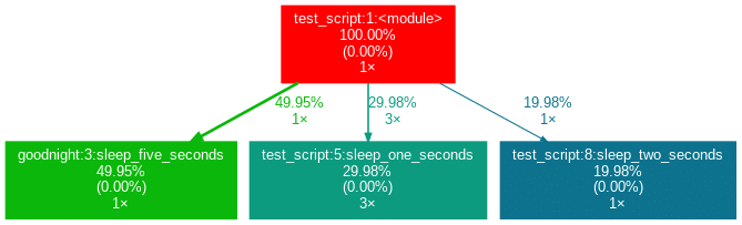
The script to be profiled always acts as a starting point and is the root of the tree. Each box is captioned with a function’s name, the overall percentage of time spent in the function, and its number of calls. The number in brackets represents the time spent in the function’s code, excluding time spent in other functions that are called in it.
In this case, all time is spent in the external module time‘s function sleep, which is why the number is 0.00%. Rarely a lot of time is spent in self-written functions, as the workload of a script usually quickly trickles down to very low-level functions of the Python implementation itself. Also, next to the arrows is the amount of time that one function passes to the other, along with the number of calls. The colors (RED-GREEN-BLUE, descending) and the thickness of the arrows indicate the relevance of different spots in the program.
Note that the percentages of the three functions above don’t add up to 100%. The reason behind is is that the graph is set up to only include self-written functions. In this case, the importing the time module caused the Python interpreter to spend 0.04% time in a function of the module importlib.
Evaluation with External Packages
Consider a second example:
# test_script_2.py

import pandas as pd
from tests.goodnight import sleep_five_seconds

# some random madness
for i in range(1000):
   a_frame = pd.DataFrame([[1,2,3]])

sleep_five_seconds()
capture this in the graph, we can add the external package (pandas) with the -x flag. However, initializing a Pandas DataFrame is done within many pandas-internal functions. Frankly, I am personally not interested in the inner convolutions of pandas which is why I want the tree to not “sprout” too deep into the pandas mechanics. This can be accounted for by allowing only functions to show up if a minimal percentage of the runtime is spent in them.
Exactly this can be done using the -mflag. In combination, project_graph -m 8 -x pandas test_script_2.py yields the following:
Toy examples aside, let’s move on to something more serious. A real-life data-science project could look like this one:
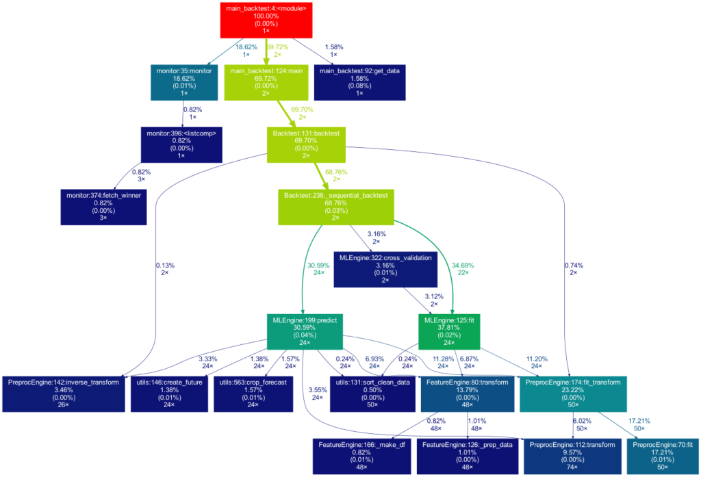
This time the tree is much bigger. It is actually even bigger than what you see in the illustration, as many more self-written functions are invoked. However, they are trimmed from the tree for clarity, as functions in which less than 0.5 % of the overall time is spent are filtered out (this is the default setting for the -m flag). Note that such a graph also really shines when searching for performance bottlenecks. One can see right away which functions carry most of the workload, when they are called, and how often they are called. This may prevent you from optimizing your program in the wrong spots while ignoring the elephant in the room.
How to Use Project Graphs
Installation
Within your project’s environment, do the following:
brew install graphviz

pip install git+https://github.com/fior-di-latte/project_graph.git
Usage
Within your project’s environment, change your current working directory to the project’s root (this is important!) and then enterfor standard usage:
project_graph myscript.pyIf your script includes an argparser, use:
project_graph "myscript.py <arg1> <arg2> (...)"If you want to see the entire graph, including all external packages, use:
project_graph -a myscript.pyIf you want to use a visibility threshold other than 1%, use:
project_graph -m <percent_value> myscript.pyFinally, if you want to include external packages into the graph, you can specify them as follows:
project_graph -x <package1> -x <package2> (...) myscript.pyConclusion & Caveats
This package has certain weaknesses, most of which can be addressed, e.g., by formatting the code into a function-based style, by trimming with the -m flag, or adding packages by using the -x flag. Generally, if something seems odd, the best first step is probably to use the -a flag to debug. Significant caveats are the following:
- It only works on Unix systems.
- It does not show a truthful graph when used with multiprocessing. The reason behind that is that cProfile is not compatible with multiprocessing. If multiprocessing is used, only the root process will be profiled, leading to false computation times in the graph. Switch to a non-parallel version of the target script.
- Profiling a script can lead to a considerable overhead computation-wise. It can make sense to scale down the work done in your script (i.e., decrease the amount of input data). If so, the time spent in the functions, of course, can be distorted massively if the functions don’t scale linearly.
- Nested functions will not show up in the graph. In particular, a decorator implicitly nests your function and will thus hide your function. That said, when using an external decorator, don’t forget to add the decorator’s package via the
-xflag (for example,project_graph -x numba myscript.py). - If your self-written function is exclusively called from an external package’s function, you must manually add the external package with the
-xflag. Otherwise, your function will not show up in the tree, as its parent is an external function and thus not considered.
Feel free to use the little package for your own project, be it for performance analysis, code introductions for new team members, or out of sheer curiosity. As for me, I find it very satisfying to see such a visualization of my projects. If you have trouble using it, don’t hesitate to hit me up on Github.
PS: If you’re looking for a similar package in R, check out Jakob’s post on flowcharts of functions.
Do you want to learn Python? Or are you an R pro and you regularly miss the important functions and commands when working with Python? Or maybe you need a little reminder from time to time while coding? That’s exactly why cheatsheets were invented!
Cheatsheets help you in all these situations. Our first cheatsheet with Python basics is the start of a new blog series, where more cheatsheets will follow in our unique STATWORX style.
So you can be curious about our series of new Python cheatsheets that will cover basics as well as packages and workspaces relevant to Data Science.
Our cheatsheets are freely available for you to download, without registration or any other paywall.
Why have we created new cheatsheets?
As an experienced R user you will search endlessly for state-of-the-art Python cheatsheets similiar to those known from R Studio.
Sure, there are a lot of cheatsheets for every topic, but they differ greatly in design and content. As soon as we use several cheatsheets in different designs, we have to reorientate ourselves again and again and thus lose a lot of time in total. For us as data scientists it is important to have uniform cheatsheets where we can quickly find the desired function or command.
We want to counteract this annoying search for information. Therefore, we would like to regularly publish new cheatsheets in a design language on our blog in the future – and let you all participate in this work relief.
What does the first cheatsheet contain?
Our first cheatsheet in this series is aimed primarily at Python novices, R users who use Python less often, or peoples who are just starting to use it. It facilitates the introduction and overview in Python.
It makes it easier to get started and get an overview of Python. Basic syntax, data types, and how to use them are introduced, and basic control structures are introduced. This way, you can quickly access the content you learned in our STATWORX Academy, for example, or recall the basics for your next programming project.
What does the STATWORX Cheatsheet Episode 2 cover?
The next cheatsheet will cover the first step of a data scientist in a new project: Data Wrangling. Also, you can expect a cheatsheet for pandas about data loading, selection, manipulation, aggregation and merging. Happy coding!
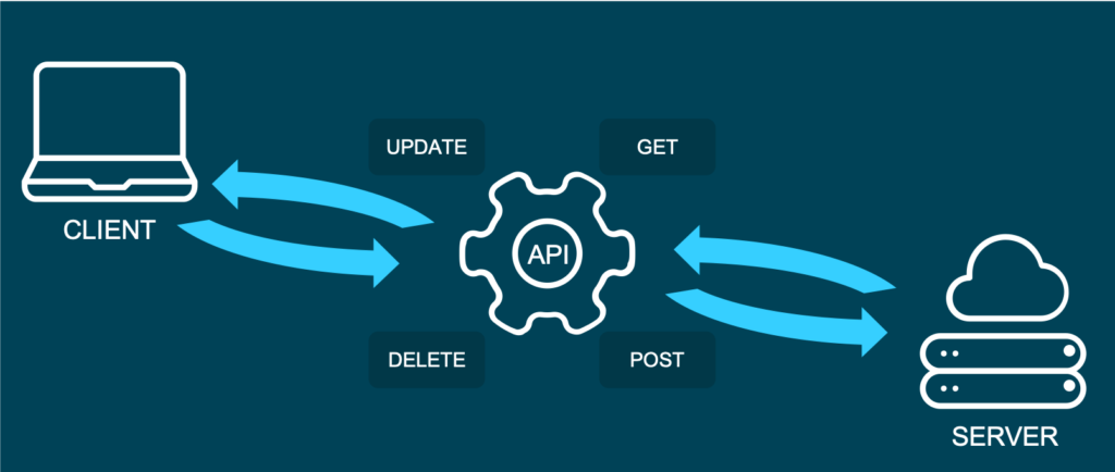
Did you ever want to make your machine learning model available to other people, but didn’t know how? Or maybe you just heard about the term API, and want to know what’s behind it? Then this post is for you!
Here at STATWORX, we use and write APIs daily. For this article, I wrote down how you can build your own API for a machine learning model that you create and the meaning of some of the most important concepts like REST. After reading this short article, you will know how to make requests to your API within a Python program. So have fun reading and learning!
What is an API?
API is short for Application Programming Interface. It allows users to interact with the underlying functionality of some written code by accessing the interface. There is a multitude of APIs, and chances are good that you already heard about the type of API, we are going to talk about in this blog post: The web API.
This specific type of API allows users to interact with functionality over the internet. In this example, we are building an API that will provide predictions through our trained machine learning model. In a real-world setting, this kind of API could be embedded in some type of application, where a user enters new data and receives a prediction in return. APIs are very flexible and easy to maintain, making them a handy tool in the daily work of a Data Scientist or Data Engineer.
An example of a publicly available machine learning API is Time Door. It provides Time Series tools that you can integrate into your applications. APIs can also be used to make data available, not only machine learning models.
And what is REST?
Representational State Transfer (or REST) is an approach that entails a specific style of communication through web services. When using some of the REST best practices to implement an API, we call that API a “REST API”. There are other approaches to web communication, too (such as the Simple Object Access Protocol: SOAP), but REST generally runs on less bandwidth, making it preferable to serve your machine learning models.
In a REST API, the four most important types of requests are:
- GET
- PUT
- POST
- DELETE
For our little machine learning application, we will mostly focus on the POST method, since it is very versatile, and lots of clients can’t send GET methods.
It’s important to mention that APIs are stateless. This means that they don’t save the inputs you give during an API call, so they don’t preserve the state. That’s significant because it allows multiple users and applications to use the API at the same time, without one user request interfering with another.
The Model
For this How-To-article, I decided to serve a machine learning model trained on the famous iris dataset. If you don’t know the dataset, you can check it out here. When making predictions, we will have four input parameters: sepal length, sepal width, petal length, and finally, petal width. Those will help to decide which type of iris flower the input is.
For this example I used the scikit-learn implementation of a simple KNN (K-nearest neighbor) algorithm to predict the type of iris:
# model.py
from sklearn import datasets
from sklearn.model_selection import train_test_split
from sklearn.neighbors import KNeighborsClassifier
from sklearn.metrics import accuracy_score
from sklearn.externals import joblib
import numpy as np


def train(X,y):

    # train test split
    X_train, X_test, y_train, y_test = train_test_split(X, y, test_size=0.3)

    knn = KNeighborsClassifier(n_neighbors=1)

    # fit the model
    knn.fit(X_train, y_train)
    preds = knn.predict(X_test)
    acc = accuracy_score(y_test, preds)
    print(f'Successfully trained model with an accuracy of {acc:.2f}')

    return knn

if __name__ == '__main__':

    iris_data = datasets.load_iris()
    X = iris_data['data']
    y = iris_data['target']

    labels = {0 : 'iris-setosa',
              1 : 'iris-versicolor',
              2 : 'iris-virginica'}

    # rename integer labels to actual flower names
    y = np.vectorize(labels.__getitem__)(y)

    mdl = train(X,y)

    # serialize model
    joblib.dump(mdl, 'iris.mdl')
As you can see, I trained the model with 70% of the data and then validated with 30% out of sample test data. After the model training has taken place, I serialize the model with the joblib library. Joblib is basically an alternative to pickle, which preserves the persistence of scikit estimators, which include a large number of numpy arrays (such as the KNN model, which contains all the training data). After the file is saved as a joblib file (the file ending thereby is not important by the way, so don’t be confused that some people call it .model or .joblib), it can be loaded again later in our application.
The API with Python and Flask
To build an API from our trained model, we will be using the popular web development package Flask and Flask-RESTful. Further, we import joblib to load our model and numpy to handle the input and output data.
In a new script, namely app.py, we can now set up an instance of a Flask app and an API and load the trained model (this requires saving the model in the same directory as the script):
from flask import Flask
from flask_restful import Api, Resource, reqparse
from sklearn.externals import joblib
import numpy as np

APP = Flask(__name__)
API = Api(APP)

IRIS_MODEL = joblib.load('iris.mdl')
The second step now is to create a class, which is responsible for our prediction. This class will be a child class of the Flask-RESTful class Resource. This lets our class inherit the respective class methods and allows Flask to do the work behind your API without needing to implement everything.
In this class, we can also define the methods (REST requests) that we talked about before. So now we implement a Predict class with a .post() method we talked about earlier.
The post method allows the user to send a body along with the default API parameters. Usually, we want the body to be in JSON format. Since this body is not delivered directly in the URL, but as a text, we have to parse this text and fetch the arguments. The flask _restful package offers the RequestParser class for that. We simply add all the arguments we expect to find in the JSON input with the .add_argument() method and parse them into a dictionary. We then convert it into an array and return the prediction of our model as JSON.
class Predict(Resource):

    @staticmethod
    def post():
        parser = reqparse.RequestParser()
        parser.add_argument('petal_length')
        parser.add_argument('petal_width')
        parser.add_argument('sepal_length')
        parser.add_argument('sepal_width')

        args = parser.parse_args()  # creates dict

        X_new = np.fromiter(args.values(), dtype=float)  # convert input to array

        out = {'Prediction': IRIS_MODEL.predict([X_new])[0]}

        return out, 200
You might be wondering what the 200 is that we are returning at the end: For APIs, some HTTP status codes are displayed when sending requests. You all might be familiar with the famous 404 - page not found code. 200 just means that the request has been received successfully. You basically let the user know that everything went according to plan.
In the end, you just have to add the Predict class as a resource to the API, and write the main function:
API.add_resource(Predict, '/predict')

if __name__ == '__main__':
    APP.run(debug=True, port='1080')
The '/predict' you see in the .add_resource() call, is the so-called API endpoint. Through this endpoint, users of your API will be able to access and send (in this case) POST requests. If you don’t define a port, port 5000 will be the default.
You can see the whole code for the app again here:
# app.py
from flask import Flask
from flask_restful import Api, Resource, reqparse
from sklearn.externals import joblib
import numpy as np

APP = Flask(__name__)
API = Api(APP)

IRIS_MODEL = joblib.load('iris.mdl')


class Predict(Resource):

    @staticmethod
    def post():
        parser = reqparse.RequestParser()
        parser.add_argument('petal_length')
        parser.add_argument('petal_width')
        parser.add_argument('sepal_length')
        parser.add_argument('sepal_width')

        args = parser.parse_args()  # creates dict

        X_new = np.fromiter(args.values(), dtype=float)  # convert input to array

        out = {'Prediction': IRIS_MODEL.predict([X_new])[0]}

        return out, 200


API.add_resource(Predict, '/predict')

if __name__ == '__main__':
    APP.run(debug=True, port='1080')
Run the API
Now it’s time to run and test our API!
To run the app, simply open a terminal in the same directory as your app.py script and run this command.
python run app.pyYou should now get a notification, that the API runs on your localhost in the port you defined. There are several ways of accessing the API once it is deployed. For debugging and testing purposes, I usually use tools like Postman. We can also access the API from within a Python application, just like another user might want to do to use your model in their code.
We use the requests module, by first defining the URL to access and the body to send along with our HTTP request:
import requests

url = 'http://127.0.0.1:1080/predict'  # localhost and the defined port + endpoint
body = {
    "petal_length": 2,
    "sepal_length": 2,
    "petal_width": 0.5,
    "sepal_width": 3
}
response = requests.post(url, data=body)
response.json()
The output should look something like this:
Out[1]: {'Prediction': 'iris-versicolor'}That’s how easy it is to include an API call in your Python code! Please note that this API is just running on your localhost. You would have to deploy the API to a live server (e.g., on AWS) for others to access it.
Conclusion
In this blog article, you got a brief overview of how to build a REST API to serve your machine learning model with a web interface. Further, you now understand how to integrate simple API requests into your Python code. For the next step, maybe try securing your APIs? If you are interested in learning how to build an API with R, you should check out this post. I hope that this gave you a solid introduction to the concept and that you will be building your own APIs immediately. Happy coding!
Getting the data in the quantity, quality and format you need is often the most challenging part of data science projects. But it’s also one, if not the most important part. That’s why my colleagues and I at STATWORX tend to spend a lot of time setting up good ETL processes. Thanks to frameworks like Airflow this isn’t just a Data Engineer prerogative anymore. If you know a bit of SQL and Python, you can orchestrate your own ETL process like a pro. Read on to find out how!
ETL does not stand for Extraterrestrial Life
At least not in Data Science and Engineering.
ETL stands for Extract, Transform, Load and describes a set of database operations. Extracting means we read the data from one or more data sources. Transforming means we clean, aggregate or combine the data to get it into the shape we want. Finally, we load it to a destination database.
Does your ETL process consist of Karen sending you an Excel sheet that you can spend your workday just scrolling down? Or do you have to manually query a database every day, tweaking your SQL queries to the occasion? If yes, venture a peek at Airflow.
How Airflow can help with ETL processes
Airflow is a python based framework that allows you to programmatically create, schedule and monitor workflows. These workflows consist of tasks and dependencies that can be automated to run on a schedule. If anything fails, there are logs and error handling facilities to help you fix it.
Using Airflow can make your workflows more manageable, transparent and efficient. And yes, I’m talking to you fellow Data Scientists! Getting access to up-to-date, high-quality data is far too important to leave it only to the Data Engineers 😉 (we still love you).
The point is, if you’re working with data, you’ll profit from knowing how to wield this powerful tool.
How Airflow works
To learn more about Airflow, check out this blog post from my colleague Marvin. It will get you up to speed quickly. Marvin explains in more detail how Airflow works and what advantages/disadvantages it has as a workflow manager. Also, he has an excellent quick-start guide with Docker.
What matters to us is knowing that Airflow’s based on DAGs or Directed Acyclic Graphs that describe what tasks our workflow consists of and how these are connected.
Note that in this tutorial we’re not actually going to deploy the pipeline. Otherwise, this post would be even longer. And you probably have friends and family that like to see you. So today is all about creating a DAG step by step.
If you care more about the deployment side of things, stay tuned though! I plan to do a step by step guide of how to do that in the next post. As a small solace, know that you can test every task of your workflow with:
airflow test [your dag id] [your task id] [execution date]There are more options, but that’s all we need for now.
What you need to follow this tutorial
This tutorial shows you how you can use Airflow in combination with BigQuery and Google Cloud Storage to run a daily ETL process. So what you need is:
- A Google Cloud account
- A python environment with Airflow
- A CSV file that I prepared for this tutorial
If you already have a Google Cloud account, you can hit the ground running! If not, consider opening one. You do need to provide a credit card. But don’t worry, this tutorial won’t cost you. If you sign up new, you get a free yearly trial period. But even if that one’s expired, we’re staying well within the bounds of Google’s Always Free Tier.
Finally, it helps if you know some SQL. I know it’s something most Data Scientists don’t find too sexy, but the more you use it the more you like it. I guess it’s like the orthopedic shoes of Data Science. A bit ugly sure, but unbeatable in what it’s designed for. If you’re not familiar with SQL or dread it like the plague, don’t sweat it. Each query’s name says what it does.
What BigQuery and Google Cloud Storage are
BigQuery and Cloud Storage are some of the most popular products of the Google Cloud Platform (GCP). BigQuery is a serverless cloud data warehouse that allows you to analyze up to petabytes of data at high speeds. Cloud Storage, on the other hand, is just that: a cloud-based object storage. Grossly simplified, we use BigQuery as a database to query and Cloud Storage as a place to save the results.
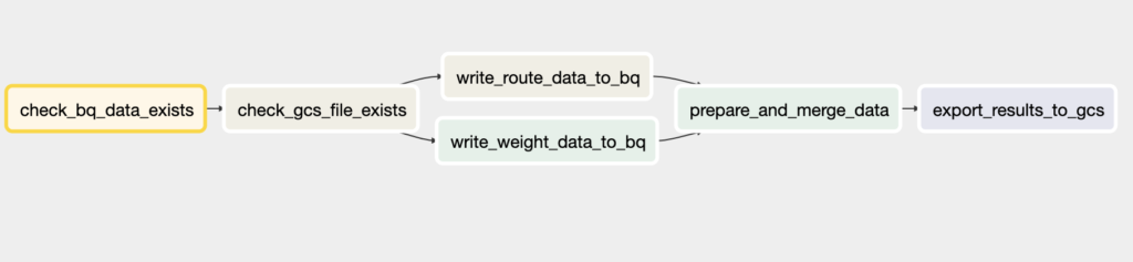
In more detail, our ETL process:
- checks for the existence of data in BigQuery and Google Cloud Storage
- queries a BigQuery source table and writes the result to a table
- ingests the Cloud Storage data into another BigQuery table
- merges the two tables and writes the result back to Cloud Storage as a CSV
Connecting Airflow to these services
If you set up a Google Cloud account you should have a JSON authentication file. I suggest putting this in your home directory. We use this file to connect Airflow to BigQuery and Cloud Storage. To do this, just copy and paste these lines in your terminal, substituting your project ID and JSON path. You can read more about connections here.
# for bigquery
airflow connections -d --conn_id bigquery_default

airflow connections -a --conn_id bigquery_default --conn_uri 'google-cloud-platform://:@:?extra__google_cloud_platform__project=[YOUR PROJECT ID]&extra__google_cloud_platform__key_path=[PATH TO YOUR JSON]'


# for google cloud storage
airflow connections -d --conn_id google_cloud_default

airflow connections -a --conn_id google_cloud_default --conn_uri 'google-cloud-platform://:@:?extra__google_cloud_platform__project=[YOUR PROJECT ID]&extra__google_cloud_platform__key_path=[PATH TO YOUR JSON]'
Writing our DAG
Task 0: Setting the start date and the schedule interval
We are ready to define our DAG! This DAG consists of multiple tasks or things our ETL process should do. Each task is instantiated by a so-called operator. Since we’re working with BigQuery and Cloud Storage, we take the appropriate Google Cloud Platform (GCP) operators.
Before defining any tasks, we specify the start date and schedule interval. The start date is the date when the DAG first runs. In this case, I picked February 20th, 2020. The schedule interval is how often the DAG runs, i.e. on what schedule. You can use cron notation here, a timedelta object or one of airflow’s cron presets (e.g. ‘@daily’).
Tip: you normally want to keep the start date static to avoid unpredictable behavior (so no datetime.now() shenanigans even though it may seem tempting).
# set start date and schedule interval
start_date = datetime(2020, 2, 20)
schedule_interval = timedelta(days=1)
You find the complete DAG file on our STATWORX Github. There you also see all the config parameters I set, e.g., what our project, dataset, buckets, and tables are called, as well as all the queries. We gloss over it here, as it’s not central to understanding the DAG.
Task 1: Check that there is data in BigQuery
We set up our DAG taking advantage of python’s context manager. You don’t have to do this, but it saves some typing. A little detail: I’m setting catchup=False because I don’t want Airflow to do a backfill on my data.
# write dag
with DAG(dag_id='blog', default_args=default_args, schedule_interval=schedule_interval, catchup=False) as dag:

    t1 = BigQueryCheckOperator(task_id='check_bq_data_exists',
                               sql=queries.check_bq_data_exists,
                               use_legacy_sql=False)
We start by checking if the data for the date we’re interested in is available in the source table. Our source table, in this case, is the Google public dataset bigquery-public-data.austin_waste.waste_and_diversion. To perform this check we use the aptly named BigQueryCheckOperator and pass it an SQL query.
If the check_bq_data_exists query returns even one non-null row of data, we consider it successful and the next task can run. Notice that we’re making use of macros and Jinja templating to dynamically insert dates into our queries that are rendered at runtime.
check_bq_data_exists = """
SELECT load_id
FROM `bigquery-public-data.austin_waste.waste_and_diversion`
WHERE report_date BETWEEN DATE('{{ macros.ds_add(ds, -365) }}') AND DATE('{{ ds }}')
"""
Task 2: Check that there is data in Cloud Storage
Next, let’s check that the CSV file is in Cloud Storage. If you’re following along, just download the file from the STATWORX Github and upload it to your bucket. We pretend that this CSV gets uploaded to Cloud Storage by another process and contains data that we need (in reality I just extracted it from the same source table).
So we don’t care how the CSV got into the bucket, we just want to know: is it there? This can easily be verified in Airflow with the GoogleCloudStorageObjectSensor which checks for the existence of a file in Cloud Storage. Notice the indent because it’s still part of our DAG context.
Defining the task itself is simple: just tell Airflow which object to look for in your bucket.
    t2 = GoogleCloudStorageObjectSensor(task_id='check_gcs_file_exists',
                                        bucket=cfg.BUCKET,
                                        object=cfg.SOURCE_OBJECT)
Task 3: Extract data and save it to BigQuery
If the first two tasks succeed, then all the data we need is available! Now let’s extract some data from the source table and save it to a new table of our own. For this purpose, there’s none better than the BigQueryOperator.
    t3 = BigQueryOperator(task_id='write_weight_data_to_bq',
                          sql=queries.write_weight_data_to_bq,
                          destination_dataset_table=cfg.BQ_TABLE_WEIGHT,
                          create_disposition='CREATE_IF_NEEDED',
                          write_disposition='WRITE_TRUNCATE',
                          use_legacy_sql=False)
This operator sends a query called write_weight_data_to_bq to BigQuery and saves the result in a table specified by the config parameter cfg.BQ_TABLE_WEIGHT. We can also set a create and write disposition if we so choose.
The query itself pulls the total weight of dead animals collected every day by Austin waste management services for a year. If the thought of possum pancakes makes you queasy, just substitute ‘RECYCLING – PAPER’ for the TYPE variable in the config file.
Task 4: Ingest Cloud Storage data into BigQuery
Once we’re done extracting the data above, we need to get the data that’s currently in our Cloud Storage bucket into BigQuery as well. To do this, just tell Airflow what (source) object from your Cloud Storage bucket should go to which (destination) table in your BigQuery dataset.
Tip: You can also specify a schema at this step, but I didn’t bother since the autodetect option worked well.
    t4 = GoogleCloudStorageToBigQueryOperator(task_id='write_route_data_to_bq',
                                              bucket=cfg.BUCKET,
                                              source_objects=[cfg.SOURCE_OBJECT],
                                              field_delimiter=';',
                                              destination_project_dataset_table=cfg.BQ_TABLE_ROUTE,
                                              create_disposition='CREATE_IF_NEEDED',
                                              write_disposition='WRITE_TRUNCATE',
                                              skip_leading_rows=1)
Task 5: Merge BigQuery and Cloud Storage data
Now we have both the BigQuery source table extract and the CSV data from Cloud Storage in two separate BigQuery tables. Time to merge them! How do we do this?
The BigQueryOperator is our friend here. We just pass it a SQL query that specifies how we want the tables merged. By specifying the destination_dataset argument, it’ll put the result into a table that we choose.
    t5 = BigQueryOperator(task_id='prepare_and_merge_data',
                          sql=queries.prepare_and_merge_data,
                          use_legacy_sql=False,
                          destination_dataset_table=cfg.BQ_TABLE_MERGE,
                          create_disposition='CREATE_IF_NEEDED',
                          write_disposition='WRITE_TRUNCATE')
Click below if you want to see the query. I know it looks long and excruciating, but trust me, there are Tinder dates worse than this (‘So, uh, do you like SQL?’ – ‘Which one?’). If he/she follows it up with Lord of the Rings or ‘Yes’, propose!
What is it that this query is doing? Let’s recap: We have two tables at the moment. One is basically a time series on how much dead animal waste Austin public services collected over the course of a year. The second table contains information on what type of routes were driven on those days.
As if this pipeline wasn’t weird enough, we now also want to know what the most common route type was on a given day. So we start by counting what route types were recorded on a given day. Next, we use a window function (... OVER (PARTITION BY ... ORDER BY ...)) to find the route type with the highest count for each day. In the end, we pull it out and using the date as a key, merge it to the table with the waste info.
prepare_and_merge_data = """
WITH
simple_route_counts AS (
SELECT report_date,
       route_type,
       count(route_type) AS count
FROM `my-first-project-238015.waste.route`
GROUP BY report_date, route_type
),
max_route_counts AS (
SELECT report_date,
       FIRST_VALUE(route_type) OVER (PARTITION BY report_date ORDER BY count DESC) AS top_route,
       ROW_NUMBER() OVER (PARTITION BY report_date ORDER BY count desc) AS row_number
FROM simple_route_counts
),
top_routes AS (
SELECT report_date AS date,
       top_route,
FROM max_route_counts
WHERE row_number = 1
)
SELECT a.date,
       a.type,
       a.weight,
       b.top_route
FROM `my-first-project-238015.waste.weight` a
LEFT JOIN top_routes b
ON a.date = b.date
ORDER BY a.date DESC
"""
Task 6: Export result to Google Cloud Storage
Let’s finish off this process by exporting our result back to Cloud Storage. By now, you’re probably guessing what the right operator is called. If you guessed BigQueryToCloudStorageOperator, you’re spot on. How to use it though? Just specify what the source table and the path (uri) to the Cloud Storage bucket are called.
    t6 = BigQueryToCloudStorageOperator(task_id='export_results_to_gcs',
                                        source_project_dataset_table=cfg.BQ_TABLE_MERGE,
                                        destination_cloud_storage_uris=cfg.DESTINATION_URI,
                                        export_format='CSV')
The only thing left to do now is to determine how the tasks relate to each other, i.e. set the dependencies. We can do this using the >> notation which I find more readable than set_upstream() or set_downstream(). But take your pick.
t1 >> t2 >> [t3, t4] >> t5 >> t6The notation above says: if data is available in the BigQuery source table, check next if data is also available in Cloud Storage. If so, go ahead, extract the data from the source table and save it to a new BigQuery table. In addition, transfer the CSV file data from Cloud Storage into a separate BigQuery table. Once those two tasks are done, merge the two newly created tables. At last, export the merged table to Cloud Storage as a CSV.
Conclusion
That’s it! Thank you very much for sticking with me to the end! Let’s wrap up what we did: we wrote a DAG file to define an automated ETL process that extracts, transforms and loads data with the help of two Google Cloud Platform services: BigQuery and Cloud Storage. Everything we needed was some Python and SQL code.
What’s next? There’s much more to explore, from using the Web UI, monitoring your workflows, dynamically creating tasks, orchestrating machine learning models, and, and, and. We barely scratched the surface here.
So check out Airflow’s official website to learn more. For now, I hope you got a better sense of the possibilities you have with Airflow and how you can harness its power to manage and automate your workflows.
References
- https://airflow.apache.org/docs/stable/
- https://cloud.google.com/blog/products/gcp/how-to-aggregate-data-for-bigquery-using-apache-airflow
- https://blog.godatadriven.com/zen-of-python-and-apache-airflow
- https://diogoalexandrefranco.github.io/about-airflow-date-macros-ds-and-execution-date/
- https://www.astronomer.io/guides/templating/
- https://medium.com/datareply/airflow-lesser-known-tips-tricks-and-best-practises-cf4d4a90f8f
Recently, some colleagues and I attended the 2-day COVID-19 hackathon #wirvsvirus, organized by the German government. Thereby, we’ve developed a great application for simulating COVID-19 curves based on estimations of governmental measure effectiveness (FlatCurver). As there are many COVID-related dashboards and visualizations out there, I thought that gathering the underlying data from a single point of truth would be a minor issue. However, I soon realized that there are plenty of different data sources, mostly relying on the Johns Hopkins University COVID-19 case data. At first, I thought that’s great, but at a second glance, I revised my initial thought. The JHU datasets have some quirky issues to it that makes it a bit cumbersome to prepare and analyze it:
- weird column names including special characters
- countries and states “in the mix”
- wide format, quite unhandy for data analysis
- import problems due to line break issues
- etc.
For all of you, who have been or are working with COVID-19 time series data and want to step up your data-pipeline game, let me tell you: we have an API for that! The API uses official data from the European Centre for Disease Prevention and Control and delivers a clear and concise data structure for further processing, analysis, etc.
Overview of our COVID-19 API
Our brand new COVID-19-API brings you the latest case number time series right into your application or analysis, regardless of your development environment. For example, you can easily import the data into Python using the requests package:
import requests
import json
import pandas as pd

# POST to API
payload = {'country': 'Germany'} # or {'code': 'DE'}
URL = 'https://api.statworx.com/covid'
response = requests.post(url=URL, data=json.dumps(payload))

# Convert to data frame
df = pd.DataFrame.from_dict(json.loads(response.text))
Or if you’re an R aficionado, use httr and jsonlite to grab the lastest data and turn it into a cool plot.
library(httr)
library(dplyr)
library(jsonlite)
library(ggplot2)

# Post to API
payload <- list(code = "ALL")
response <- httr::POST(url = "https://api.statworx.com/covid",
                       body = toJSON(payload, auto_unbox = TRUE), encode = "json")

# Convert to data frame
content <- rawToChar(response$content)
df <- data.frame(fromJSON(content))

# Make a cool plot
df %>%
  mutate(date = as.Date(date)) %>%
  filter(cases_cum > 100) %>%
  filter(code %in% c("US", "DE", "IT", "FR", "ES")) %>%
  group_by(code) %>%
  mutate(time = 1:n()) %>%
  ggplot(., aes(x = time, y = cases_cum, color = code)) +
  xlab("Days since 100 cases") + ylab("Cumulative cases") +
  geom_line() + theme_minimal()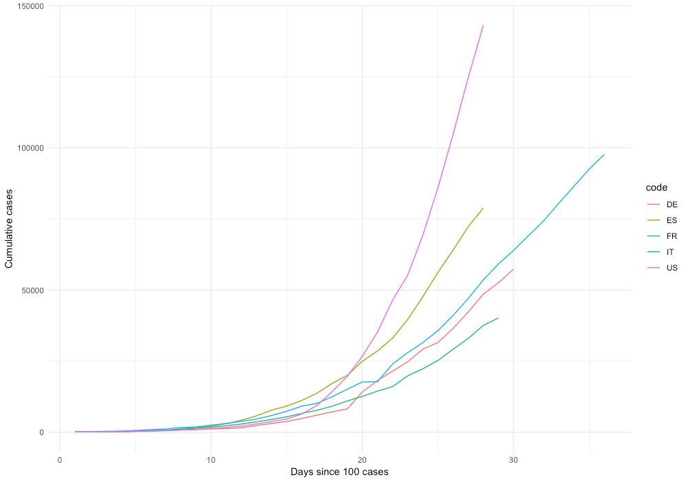
Developing the API using Flask
Developing a simple web app using Python is straightforward using Flask. Flask is a web framework for Python. It allows you to create websites, web applications, etc. right from Python. Flask is widely used to develop web services and APIs. A simple Flask app looks something like this.
from flask import Flask
app = Flask(__name__)

@app.route('/')
def handle_request():
  """ This code gets executed """
  return 'Your first Flask app!'
In the example above, app.route decorator defines at which URL our function should be triggered. You can specify multiple decorators to trigger different functions for each URL. You might want to check out our code in the Github repository to see how we build the API using Flask.
Deployment using Google Cloud Run
Developing the API using Flask is straightforward. However, building the infrastructure and auxiliary services around it can be challenging, depending on your specific needs. A couple of things you have to consider when deploying an API:
- Authentification
- Security
- Scalability
- Latency
- Logging
- Connectivity
We’ve decided to use Google Cloud Run, a container-based serverless computing framework on Google Cloud. Basically, GCR is a fully managed Kubernetes service, that allows you to deploy scalable web services or other serverless functions based on your container. This is how our Dockerfile looks like.
# Use the official image as a parent image
FROM python:3.7
# Copy the file from your host to your current location
COPY ./main.py /app/main.py
COPY ./requirements.txt /app/requirements.txt
# Set the working directory
WORKDIR /app
# Run the command inside your image filesystem
RUN pip install -r requirements.txt
# Inform Docker that the container is listening on the specified port at runtime.
EXPOSE 80
# Run the specified command within the container.
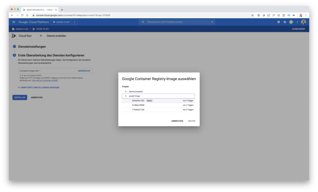
CMD ["python", "main.py"]You can develop your container locally and then push it in to the container registry of your GCP project. To do so, you have to tag your local image using docker tag according to the following scheme: [HOSTNAME]/[PROJECT-ID]/[IMAGE]. The hostname is one of the following: gcr.io, us.gcr.io, eu.gcr.io, asia.gcr.io. Afterward, you can push using gcloud push, followed by your image tag. From there, you can easily connect the container to the Google Cloud Run service:
When deploying the service, you can define parameters for scaling, etc. However, this is not in scope for this post. Furthermore, GCR allows custom domain mapping to functions. That’s why we have the neat API endpoint https://api.statworx.com/covid.
Conclusion
Building and deploying a web service is easier than ever. We hope that you find our new API useful for your projects and analyses regarding COVID-19. If you have any questions or remarks, feel free to contact us or to open an issue on Github. Lastly, if you make use of our free API, please add a link to our website, https://statworx-1727.demosrv.dev to your project. Thanks in advance and stay healthy!
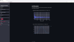
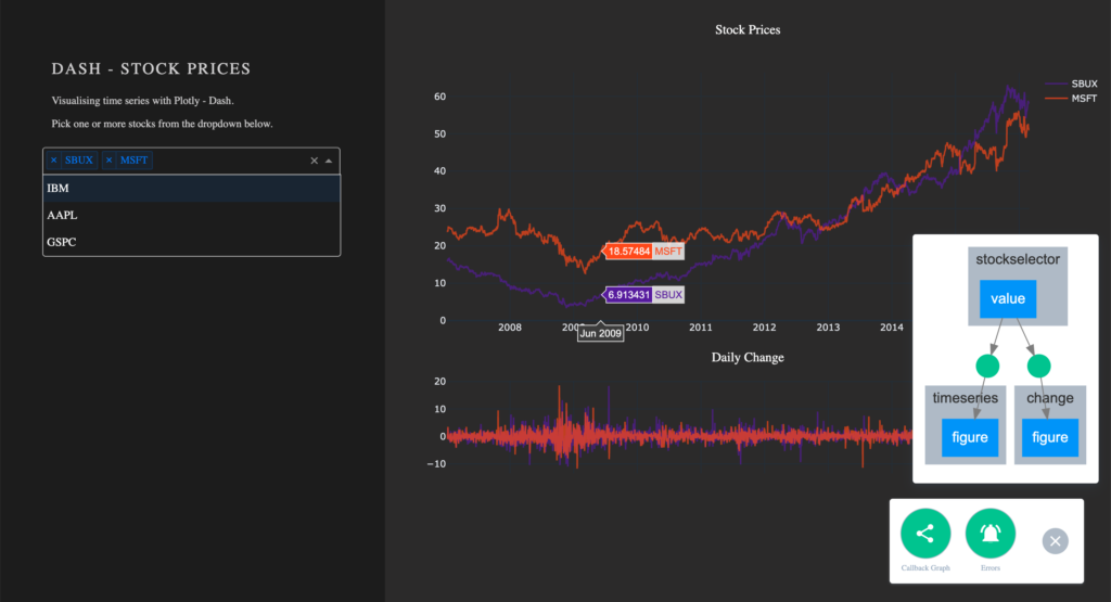
From my experience here at STATWORX, the best way to learn something is by trying it out yourself – with a little help from a friend! In this article, I will focus on giving you a hands-on guide on how to build a dashboard in Python. As a framework, we will be using Dash, and the goal is to create a basic dashboard with a dropdown and two reactive graphs:
Developed as an open-source library by Plotly, the Python framework Dash is built on top of Flask, Plotly.js, and React.js. Dash allows the building of interactive web applications in pure Python and is particularly suited for sharing insights gained from data.
In case you’re interested in interactive charting with Python, I highly recommend my colleague Markus’ blog post Plotly – An Interactive Charting Library
For our purposes, a basic understanding of HTML and CSS can be helpful. Nevertheless, I will provide you with external resources and explain every step thoroughly, so you’ll be able to follow the guide.
The source code can be found on GitHub.
Prerequisites
The project comprises a style sheet called style.css, sample stock data stockdata2.csv and the actual Dash application app.py
Load the Stylesheet
If you want your dashboard to look like the one above, please download the file style.css from our STATWORX GitHub. That is completely optional and won’t affect the functionalities of your app. Our stylesheet is a customized version of the stylesheet used by the Dash Uber Rides Demo. Dash will automatically load any .css-file placed in a folder named assets.
dashapp
    |--assets
        |-- style.css
    |--data
        |-- stockdata2.csv
    |-- app.py
The documentation on external resources in dash can be found here.
Load the Data
Feel free to use the same data we did (stockdata2.csv), or any pick any data with the following structure:
| date | stock | value | change |
|---|---|---|---|
| 2007-01-03 | MSFT | 23.95070 | -0.1667 |
| 2007-01-03 | IBM | 80.51796 | 1.0691 |
| 2007-01-03 | SBUX | 16.14967 | 0.1134 |
import pandas as pd

# Load data
df = pd.read_csv('data/stockdata2.csv', index_col=0, parse_dates=True)
df.index = pd.to_datetime(df['Date'])
Getting Started – How to start a Dash app
After installing Dash (instructions can be found here), we are ready to start with the application. The following statements will load the necessary packages dash and dash_html_components. Without any layout defined, the app won’t start. An empty html.Div will suffice to get the app up and running.
import dash
import dash_html_components as html
If you have already worked with the WSGI web application framework Flask, the next step will be very familiar to you, as Dash uses Flask under the hood.
# Initialise the app
app = dash.Dash(__name__)

# Define the app
app.layout = html.Div()
# Run the app
if __name__ == '__main__':
    app.run_server(debug=True)
How a .css-files changes the layout of an app
The module dash_html_components provides you with several html components, also check out the documentation.
Worth to mention is that the nesting of components is done via the children attribute.
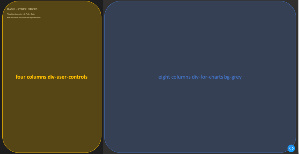
app.layout = html.Div(children=[
                      html.Div(className='row',  # Define the row element
                               children=[
                                  html.Div(className='four columns div-user-controls'),  # Define the left element
                                  html.Div(className='eight columns div-for-charts bg-grey')  # Define the right element
                                  ])
                                ])
The first html.Div() has one child. Another html.Div named row, which will contain all our content. The children of row are four columns div-user-controls and eight columns div-for-charts bg-grey.
The style for these div components come from our style.css.
Now let’s first add some more information to our app, such as a title and a description. For that, we use the Dash Components H2 to render a headline and P to generate html paragraphs.
children = [
    html.H2('Dash - STOCK PRICES'),
    html.P('''Visualising time series with Plotly - Dash'''),
    html.P('''Pick one or more stocks from the dropdown below.''')
]
Switch to your terminal and run the app with python app.py.

The basics of an app’s layout
Another nice feature of Flask (and hence Dash) is hot-reloading. It makes it possible to update our app on the fly without having to restart the app every time we make a change to our code.
Running our app with debug=True also adds a button to the bottom right of our app, which lets us take a look at error messages, as well a Callback Graph. We will come back to the Callback Graph in the last section of the article when we’re done implementing the functionalities of the app.
Charting in Dash – How to display a Plotly-Figure
With the building blocks for our web app in place, we can now define a plotly-graph. The function dcc.Graph() from dash_core_components uses the same figure argument as the plotly package. Dash translates every aspect of a plotly chart to a corresponding key-value pair, which will be used by the underlying JavaScript library Plotly.js.
In the following section, we will need the express version of plotly.py, as well as the Package Dash Core Components. Both packages are available with the installation of Dash.
import dash_core_components as dcc
import plotly.express as px
Dash Core Components has a collection of useful and easy-to-use components, which add interactivity and functionalities to your dashboard.
Plotly Express is the express-version of plotly.py, which simplifies the creation of a plotly-graph, with the drawback of having fewer functionalities.
To draw a plot on the right side of our app, add a dcc.Graph() as a child to the html.Div() named eight columns div-for-charts bg-grey. The component dcc.Graph() is used to render any plotly-powered visualization. In this case, it’s figure will be created by px.line() from the Python package plotly.express. As the express version of Plotly has limited native configurations, we are going to change the layout of our figure with the method update_layout(). Here, we use rgba(0, 0, 0, 0) to set the background transparent. Without updating the default background- and paper color, we would have a big white box in the middle of our app. As dcc.Graph() only renders the figure in the app; we can’t change its appearance once it’s created.
dcc.Graph(id='timeseries',
config={'displayModeBar': False},
animate=True,
figure=px.line(df,
x='Date',
y='value',
color='stock',
template='plotly_dark').update_layout(
{'plot_bgcolor': 'rgba(0, 0, 0, 0)',
'paper_bgcolor': 'rgba(0, 0, 0, 0)'})
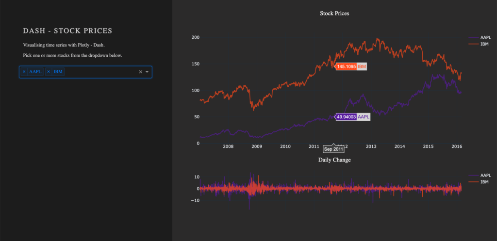
)After Dash reload the application, you will end up in something like that: A dashboard with a plotted graph:
Creating a Dropdown Menu
Another core component is dcc.dropdown(), which is used – you’ve guessed it – to create a dropdown menu. The available options in the dropdown menu are either given as arguments or supplied by a function. For our dropdown menu, we need a function that returns a list of dictionaries. The list contains dictionaries with two keys, label and value. These dictionaries provide the available options to the dropdown menu. The value of label is displayed in our app. The value of value will be exposed for other functions to use, and should not be changed. If you prefer the full name of a company to be displayed instead of the short name, you can do so by changing the value of the key label to Microsoft. For the sake of simplicity, we will use the same value for the keys label and value.
Add the following function to your script, before defining the app’s layout.
# Creates a list of dictionaries, which have the keys 'label' and 'value'.
def get_options(list_stocks):
    dict_list = []
    for i in list_stocks:
        dict_list.append({'label': i, 'value': i})

    return dict_list
With a function that returns the names of stocks in our data in key-value pairs, we can now add dcc.Dropdown() from the Dash Core Components to our app. Add a html.Div() as child to the list of children of four columns div-user-controls, with the argument className=div-for-dropdown. This html.Div() has one child, dcc.Dropdown().
We want to be able to select multiple stocks at the same time and a selected default value, so our figure is not empty on startup. Set the argument multi=True and chose a default stock for value.
 html.Div(className='div-for-dropdown',
          children=[
              dcc.Dropdown(id='stockselector',
                           options=get_options(df['stock'].unique()),
                           multi=True,
                           value=[df['stock'].sort_values()[0]],
                           style={'backgroundColor': '#1E1E1E'},
                           className='stockselector')
                    ],
          style={'color': '#1E1E1E'})
The id and options arguments in dcc.Dropdown() will be important in the next section. Every other argument can be changed. If you want to try out different styles for the dropdown menu, follow the link for a list of different dropdown menus.
Working with Callbacks
How to add interactive functionalities to your app
Callbacks add interactivity to your app. They can take inputs, for example, certain stocks selected via a dropdown menu, pass these inputs to a function and pass the return value of the function to another component. We will write a function that returns a figure based on provided stock names. A callback will pass the selected values from the dropdown to the function and return the figure to a dcc.Grapph() in our app.
At this point, the selected values in the dropdown menu do not change the stocks displayed in our graph. For that to happen, we need to implement a callback. The callback will handle the communication between our dropdown menu 'stockselector' and our graph 'timeseries'. We can delete the figure we have previously created, as we won’t need it anymore.
We want two graphs in our app, so we will add another dcc.Graph() with a different id.
- Remove the
figureargument fromdcc.Graph(id='timeseries') - Add another
dcc.Graph()withclassName='change'as child to thehtml.Div()namedeight columns div-for-charts bg-grey.
dcc.Graph(id='timeseries', config={'displayModeBar': False})
dcc.Graph(id='change', config={'displayModeBar': False})
Callbacks add interactivity to your app. They can take Inputs from components, for example certain stocks selected via a dropdown menu, pass these inputs to a function and pass the returned values from the function back to components.
In our implementation, a callback will be triggered when a user selects a stock. The callback uses the value of the selected items in the dropdown menu (Input) and passes these values to our functions update_timeseries() and update_change(). The functions will filter the data based on the passed inputs and return a plotly figure from the filtered data. The callback then passes the figure returned from our functions back to the component specified in the output.
A callback is implemented as a decorator for a function. Multiple inputs and outputs are possible, but for now, we will start with a single input and a single output. We need the class dash.dependencies.Input and dash.dependencies.Output.
Add the following line to your import statements.
from dash.dependencies import Input, OutputInput() and Output() take the id of a component (e.g. in dcc.Graph(id='timeseries') the components id is 'timeseries') and the property of a component as arguments.
Example Callback:
# Update Time Series
@app.callback(Output('id of output component', 'property of output component'),
              [Input('id of input component', 'property of input component')])
def arbitrary_function(value_of_first_input):
    '''
    The property of the input component is passed to the function as value_of_first_input.
    The functions return value is passed to the property of the output component.
    '''
    return arbitrary_output
If we want our stockselector to display a time series for one or more specific stocks, we need a function. The value of our input is a list of stocks selected from the dropdown menu stockselector.
Implementing Callbacks
The function draws the traces of a plotly-figure based on the stocks which were passed as arguments and returns a figure that can be used by dcc.Graph(). The inputs for our function are given in the order in which they were set in the callback. Names chosen for the function’s arguments do not impact the way values are assigned.
Update the figure time series:
@app.callback(Output('timeseries', 'figure'),
              [Input('stockselector', 'value')])
def update_timeseries(selected_dropdown_value):
    ''' Draw traces of the feature 'value' based one the currently selected stocks '''
    # STEP 1
    trace = []
    df_sub = df
    # STEP 2
    # Draw and append traces for each stock
    for stock in selected_dropdown_value:
        trace.append(go.Scatter(x=df_sub[df_sub['stock'] == stock].index,
                                 y=df_sub[df_sub['stock'] == stock]['value'],
                                 mode='lines',
                                 opacity=0.7,
                                 name=stock,
                                 textposition='bottom center'))
    # STEP 3
    traces = [trace]
    data = [val for sublist in traces for val in sublist]
    # Define Figure
    # STEP 4
    figure = {'data': data,
              'layout': go.Layout(
                  colorway=["#5E0DAC", '#FF4F00', '#375CB1', '#FF7400', '#FFF400', '#FF0056'],
                  template='plotly_dark',
                  paper_bgcolor='rgba(0, 0, 0, 0)',
                  plot_bgcolor='rgba(0, 0, 0, 0)',
                  margin={'b': 15},
                  hovermode='x',
                  autosize=True,
                  title={'text': 'Stock Prices', 'font': {'color': 'white'}, 'x': 0.5},
                  xaxis={'range': [df_sub.index.min(), df_sub.index.max()]},
              ),

              }

    return figure
STEP 1
- A
tracewill be drawn for each stock. Create an emptylistfor each trace from the plotly figure.
STEP 2
Within the for-loop, a trace for a plotly figure will be drawn with the function go.Scatter().
- Iterate over the stocks currently selected in our dropdown menu, draw a trace, and append that trace to our list from step 1.
STEP 3
- Flatten the traces
STEP 4
Plotly figures are dictionaries with the keys data and layout. The value of data is our flattened list with the traces we have drawn. The layout is defined with the plotly class go.Layout().
- Add the trace to our figure
- Define the layout of our figure
Now we simply repeat the steps above for our second graph. Just change the data for our y-Axis to change and slightly adjust the layout.
Update the figure change:
@app.callback(Output('change', 'figure'),
              [Input('stockselector', 'value')])
def update_change(selected_dropdown_value):
    ''' Draw traces of the feature 'change' based one the currently selected stocks '''
    trace = []
    df_sub = df
    # Draw and append traces for each stock
    for stock in selected_dropdown_value:
        trace.append(go.Scatter(x=df_sub[df_sub['stock'] == stock].index,
                                 y=df_sub[df_sub['stock'] == stock]['change'],
                                 mode='lines',
                                 opacity=0.7,
                                 name=stock,
                                 textposition='bottom center'))
    traces = [trace]
    data = [val for sublist in traces for val in sublist]
    # Define Figure
    figure = {'data': data,
              'layout': go.Layout(
                  colorway=["#5E0DAC", '#FF4F00', '#375CB1', '#FF7400', '#FFF400', '#FF0056'],
                  template='plotly_dark',
                  paper_bgcolor='rgba(0, 0, 0, 0)',
                  plot_bgcolor='rgba(0, 0, 0, 0)',
                  margin={'t': 50},
                  height=250,
                  hovermode='x',
                  autosize=True,
                  title={'text': 'Daily Change', 'font': {'color': 'white'}, 'x': 0.5},
                  xaxis={'showticklabels': False, 'range': [df_sub.index.min(), df_sub.index.max()]},
              ),
              }

    return figure
Run your app again. You are now able to select one or more stocks from the dropdown. For each selected item, a line plot will be generated in the graph. By default, the dropdown menu has search functionalities, which makes the selection out of many available options an easy task.
Visualize Callbacks – Callback Graph
With the callbacks in place and our app completed, let’s take a quick look at our callback graph. If you are running your app with debug=True, a button will appear in the bottom right corner of the app. Here we have access to a callback graph, which is a visual representation of the callbacks which we have implemented in our code. The graph shows that our components timeseries and change display a figure based on the value of the component stockselector. If your callbacks don’t work how you expect them to, especially when working on larger and more complex apps, this tool will come in handy.
Conclusion
Let’s recap the most important building blocks of Dash. Getting the App up and running requires just a couple lines of code. A basic understanding of HTML and CSS is enough to create a simple Dash dashboard. You don’t have to worry about creating interactive charts, Plotly already does that for you. Making your dashboard reactive is done via Callbacks, which are functions with the users’ interaction as the input.
If you liked this blog, feel free to contact me via LinkedIn or Email. I am curious to know what you think and always happy to answer any questions about data, my journey to data science, or the exciting things we do here at STATWORX.
Thank you for reading!
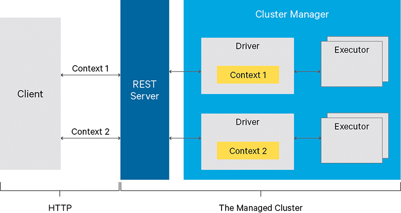
Livy is a REST web service for submitting Spark Jobs or accessing – and thus sharing – long-running Spark Sessions from a remote place. Instead of tedious configuration and installation of your Spark client, Livy takes over the work and provides you with a simple and convenient interface.
We at STATWORX use Livy to submit Spark Jobs from Apache’s workflow tool Airflow on volatile Amazon EMR cluster. Besides, several colleagues with different scripting language skills share a running Spark cluster.
Another great aspect of Livy, namely, is that you can choose from a range of scripting languages: Java, Scala, Python, R. As it is the case for Spark, which one of them you actually should/can use, depends on your use case (and on your skills).
Apache Livy is still in the Incubator state, and code can be found at the Git project.
When you should use it
Since REST APIs are easy to integrate into your application, you should use it when:
- multiple clients want to share a Spark Session.
- the clients are lean and should not be overloaded with installation and configuration.
- you need a quick setup to access your Spark cluster.
- you want to Integrate Spark into an app on your mobile device.
- you have volatile clusters, and you do not want to adapt configuration every time.
- a remote workflow tool submits spark jobs.
Preconditions
Livy is generally user-friendly, and you do not really need too much preparation. All you basically need is an HTTP client to communicate to Livy’s REST API. REST APIs are known to be easy to access (states and lists are accessible even by browsers), HTTP(s) is a familiar protocol (status codes to handle exceptions, actions like GET and POST, etc.) while providing all security measures needed.
Since Livy is an agent for your Spark requests and carries your code (either as script-snippets or packages for submission) to the cluster, you actually have to write code (or have someone writing the code for you or have a package ready for submission at hand).
I opted to maily use python as Spark script language in this blog post and to also interact with the Livy interface itself. Some examples were executed via curl, too.
How to use Livy
There are two modes to interact with the Livy interface:
- Interactive Sessions have a running session where you can send statements over. Provided that resources are available, these will be executed, and output can be obtained. It can be used to experiment with data or to have quick calculations done.
- Jobs/Batch submit code packages like programs. A typical use case is a regular task equipped with some arguments and workload done in the background. This could be a data preparation task, for instance, which takes input and output directories as parameters.
In the following, we will have a closer look at both cases and the typical process of submission. Each case will be illustrated by examples.
Interactive Sessions
Let’s start with an example of an interactive Spark Session. Throughout the example, I use python and its requests package to send requests to and retrieve responses from the REST API. As mentioned before, you do not have to follow this path, and you could use your preferred HTTP client instead (provided that it also supports POST and DELETE requests).
Starting with a Spark Session. There is a bunch of parameters to configure (you can look up the specifics at Livy Documentation), but for this blog post, we stick to the basics, and we will specify its name and the kind of code. If you have already submitted Spark code without Livy, parameters like executorMemory, (YARN) queue might sound familiar, and in case you run more elaborate tasks that need extra packages, you will definitely know that the jars parameter needs configuration as well.
To initiate the session we have to send a POST request to the directive /sessions along with the parameters.
import requests
LIVY_HOST = 'http://livy-server'

directive = '/sessions'
headers = {'Content-Type': 'application/json'}

data = {'kind':'pyspark','name':'first-livy'}

resp = requests.post(LIVY_HOST+directive, headers=headers, data=json.dumps(data))

if resp.status_code == requests.codes.created:
    session_id = resp.json()['id']
else:
    raise CustomError()
Livy, in return, responds with an identifier for the session that we extract from its response.
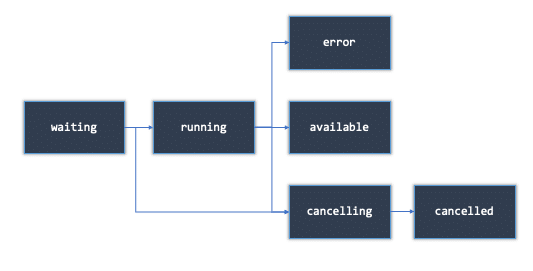
Note that the session might need some boot time until YARN (a resource manager in the Hadoop world) has allocated all the resources. Meanwhile, we check the state of the session by querying the directive: /sessions/{session_id}/state. Once the state is idle, we are able to execute commands against it.
To execute spark code, statements are the way to go. The code is wrapped into the body of a POST request and sent to the right directive: sessions/{session_id}/statements.
directive = f'/sessions/{session_id}/statements'

data = {'code':'...'}

resp = request.post(LIVY_HOST+directive, headers=headers, data=json.dumps(data))
As response message, we are provided with the following attributes:
| attribute | meaning |
|---|---|
| id | to identify the statement |
| code | the code, once again, that has been executed |
| state | the state of the execution |
| output | the output of the statement |
The statement passes some states (see below) and depending on your code, your interaction (statement can also be canceled) and the resources available, it will end up more or less likely in the success state. The crucial point here is that we have control over the status and can act correspondingly.
By the way, cancelling a statement is done via GET request /sessions/{session_id}/statements/{statement_id}/cancel
It is time now to submit a statement: Let us imagine to be one of the classmates of Gauss and being asked to sum up the numbers from 1 to 1000. Luckily you have access to a spark cluster and – even more luckily – it has the Livy REST API running which we are connected to via our mobile app: what we just have to do is write the following spark code:
import textwrap

code = textwrap.dedent("""df = spark.createDataFrame(list(range(1,1000)),'int')
df.groupBy().sum().collect()[0]['sum(value)']""")

code_packed = {'code':code}
This is all the logic we need to define. The rest is the execution against the REST API:
import time

directive = f'/sessions/{session_id}/statements'
resp = requests.post(LIVY_HOST+directive, headers=headers, data=json.dumps(code_packed))
if resp.status_code == requests.codes.created:
    stmt_id = resp.json()['id']

    while True:
        info_resp = requests.get(LIVY_HOST+f'/sessions/{session_id}/statements/{stmt_id}')
        if info_resp.status_code == requests.codes.ok:
            state = info_resp.json()['state']
                if state in ('waiting','running'):
                    time.sleep(2)
                elif state in ('cancelling','cancelled','error'):
                    raise CustomException()
                else:
                    break
        else:
            raise CustomException()
    print(info_resp.json()['output'])

else:
  #something went wrong with creation
  raise CustomException()
Every 2 seconds, we check the state of statement and treat the outcome accordingly: So we stop the monitoring as soon as state equals available. Obviously, some more additions need to be made: probably error state would be treated differently to the cancel cases, and it would also be wise to set up a timeout to jump out of the loop at some point in time.
Assuming the code was executed successfully, we take a look at the output attribute of the response:
{'status': 'ok', 'execution_count': 2, 'data': {'text/plain': '499500'}}There we go, the answer is 499500.
Finally, we kill the session again to free resources for others:
directive = f'/sessions/{session_id}/statements'
requests.delete(LIVY_HOST+directive)
Job Submission
We now want to move to a more compact solution. Say we have a package ready to solve some sort of problem packed as a jar or as a python script. What only needs to be added are some parameters – like input files, output directory, and some flags.
For the sake of simplicity, we will make use of the well known Wordcount example, which Spark gladly offers an implementation of: Read a rather big file and determine how often each word appears. We again pick python as Spark language. This time curl is used as an HTTP client.
As an example file, I have copied the Wikipedia entry found when typing in Livy. The text is actually about the roman historian Titus Livius.
I have moved to the AWS cloud for this example because it offers a convenient way to set up a cluster equipped with Livy, and files can easily be stored in S3 by an upload handler. Let’s now see, how we should proceed:
curl -X POST --data '{"file":"s3://livy-example/wordcount.py","args":[s3://livy-example/livy_life.txt"]}'
-H "Content-Type: application/json" http://livy-server:8998/batches
The structure is quite similar to what we have seen before. By passing over the batch to Livy, we get an identifier in return along with some other information like the current state.
{"id":1,"name":null,"state":"running","appId":"application_1567416002081_0005",...}To monitor the progress of the job, there is also a directive to call: /batches/{batch_id}/state
Most probably, we want to guarantee at first that the job ran successfully. In all other cases, we need to find out what has happened to our job. The directive /batches/{batchId}/log can be a help here to inspect the run.
Finally, the session is removed by:
curl -X DELETE http://livy-server:8998/batches/1 which returns: {"msg":"deleted"} and we are done.
Trivia
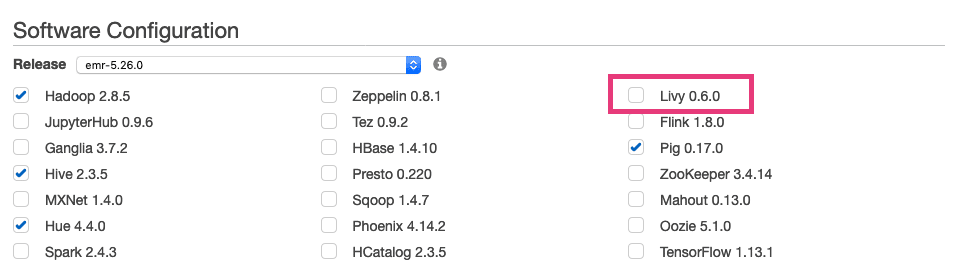
- AWS’ Hadoop cluster service EMR supports Livy natively as Software Configuration option.
- Apache’s notebook tool Zeppelin supports Livy as an Interpreter, i.e. you write code within the notebook and execute it directly against Livy REST API without handling HTTP yourself.
- Be cautious not to use Livy in every case when you want to query a Spark cluster: Namely, In case you want to use Spark as Query backend and access data via Spark SQL, rather check out Thriftserver instead of building around Livy.
- Kerberos can be integrated into Livy for authentication purposes.
My blog post aims at aspiring data scientists who have to decide which programming language they want to learn first. At STATWORX, we primarily use the two most popular languages, R and Python. Both languages have their strengths and weaknesses, which is why you should ideally master both. To get started, however, we recommend to learn one language and then tackle the other one. Don’t forget that both languages are just a tool; what matters is what you do with your tool at hand. Once you have understood and mastered the concepts of working with data, it should generally be easier to learn the second language. This blog post introduces both languages to beginners. I try to stay as unbiased as possible. For certain tasks, I prefer R – for others Python. Hence, the recommendations are subjective to my preferences. Nevertheless, I hope my experiences help you as a newcomer.
Overview R and Python
Both Python and R are open source programming languages, which means that the source code is publicly available and can be used for free. While Python is a general-purpose programming language, R was developed for statistical analysis. Therefore, users of these languages often have different backgrounds. In general terms, software developers use Python and statisticians R.
| R | Python | |
|---|---|---|
| Release | 1993 | 1991 |
| Developer | R Core Team | Python Software Foundation |
| Package Management | CRAN | PyPI |
A collection of extensions
Both languages have a basic set of functions that can be extended with packages.
The Comprehensive R Archive Network (CRAN) is a platform for R packages. A set of requirements must be satisfied to include a package on CRAN. CRAN ensures that all packages available for download work. More than 10,000 packages are available on CRAN. Since R is the standard language for statisticians, CRAN has a suitable solution for almost any statistical problem. So it’s just the right place for the latest statistical methods and analyses. Some packages depend on other packages, which can cause problems in specific scenarios. The objective of the packrat package is to ensure that all dependencies are met and everything runs smoothly.
Python has two package management platforms: conda and PyPI (Python Package Index). There are also over 10,000 packages for Python, which, compared to R, cover a vast range of applications. However, only a small share of packages are relevant for data science projects. Because complications can occur when you install Python packages globally, you can use virtual environments. They ensure smooth processes for the various packages and dependencies from package to package, similar to the packrat package in R. It can be quite hard for beginners to get a good grasp of the idea behind the different environments.
Although R and Python packages are used the same way, there are some fundamental differences. Usually, an R package is developed by a single person or a small group of researchers. The authors write the package based on a scientific paper and refer to it in the documentation. Whereas, often, large groups of developers are working on Python packages (numpy, pandas, scikit-learn).
That has advantages and disadvantages:
- The namespace for functions is clear, and functions have the same structure. E.g., when setting up different models and comparing their performance, you’ll use the scikit-learn package in Python. In R you’ll use different packages depending on what model you want to implement. The function and argument names differ from package to package – which can be cumbersome. It is noteworthy that the packages caret and parsnip are trying to correct those discrepancies in R in hindsight.
- In some cases, the functions of scikit-learn have to be checked thoroughly. The developers are usually optimization oriented and are neglecting some statistical aspects. E.g., the scikit-learn function performing a logistic regression (sklearn.linear_model.LogisticRegression) uses per default L2 regularization. The only way to get a linear logistic model without regularization is to set the regularization parameter to a high number. That’s surprising, given the functions name. Furthermore, the developers didn’t understand why this poses an issue to the users. Even if the regularized model generalizes better and, thus, might have a better predictive performance, there are cases where I would like to obtain the non-regularized coefficients for inference.
Find your IDE
Programmers often use an integrated development environment (IDE) that facilitates their work with small but subtle tools.
For R users, RStudio has become the standard IDE. The IDE is distributed by the company RStudio Inc., which stands commercially behind R. RStudio provides not only a pleasant working environment but also develops packages and extensions for the R language. For example, the RStudio team contributed important packages like tidyverse, packrat, and devtools, as well as popular extensions like shiny (for dashboards) and RMarkdown (for reports).
Python users can choose between numerous IDEs (PyCharm, Visual Studio Code, Spyder, and many more). However, no company stands behind Python and is comparable to RStudio Inc. Thanks to the efforts of the large community and the Python Software Foundation, new extensions for Python are continually being published.
The Art of Data Visualization
The most commonly used packages for data visualization with Python are matplotlib and seaborn. Dashboards can be created in Python with dash.
However, R has an ace up its sleeve in data visualization: the ggplot2 package, which is based on Leland Wilkinson’s book The Grammar of Graphics. With this package, you can create attractive and customized graphics, which you can share via shiny dashboards with others.
Both programming languages offer the possibility to create beautiful graphics easily. Nevertheless, the R package ggplot2 convinces with its flexibility, visual possibilities, and thought-out philosophy behind it. Sharing the graphics with a shiny dashboard is extremely easy. I want to mention that there are efforts to implement ggplot2 into Python.
Props for readability
Python was designed following the motto readability counts. So even people, who are not familiar with the programming language can interpret what was done in the code.
R, as a programming language, has changed a lot in recent years. Mainly because of the packages developed by the RStudio team. The readability of the code has improved substantially with the dplyr package and the use of the pipe operator, where code can be read from left to right.
The speed with different observation sizes
Next, I compare how long it takes to create a simulated dataset in R and Python. For a fair comparison, the conditions should be approximately the same. The data is simulated with the packages Xy and XyPy in R and Python, respectively. I used microbenchmark in R and timeit in Python to measure the time. Also, I parallelized the process using eight cores (R: parallel, Python: multiprocessing) to generate the simulation as fast as possible.
For the experiment, a dataset with 100 observations and 50 variables is simulated 100 times. The time it takes the computer to perform the simulation is measured individually for each simulation. That is then repeated for 1,000, 10,000, 100,000 and 1,000,000 observations.
The R and Python code snippets are shown below.
# R
# devtools::install_github("andrebleier/Xy")
# install.packages("parallel")
# install.packages("microbenchmark")

# Load packages
library(Xy)
library(microbenchmark)
library(parallel)

# Extract function definition from for loop
sim_this <- function(n_sim) {
  sim <- microbenchmark(Xy(n = n_sim,
                           numvars = c(50,0),
                           catvars = 0),
                        times = 100, unit = "s")
  data.frame(n = n_sim,
             mean = summary(sim)[, 4])
}

# Time measurement for different number of simulations
n_sim <- c(1e2, 1e3, 1e4, 1e5, 1e6)
sim_in_r <- data.frame(n = rep(0, length(n_sim)),
                       t = rep(0, length(n_sim)))
for(i in 1:length(n_sim)){
  out <- mclapply(n_sim[i],
                  FUN = sim_this,
                  mc.cores = 8)

  sim_in_r[i, 1] <- out[[1]][1]
  sim_in_r[i, 2] <- out[[1]][2]
}
# Python
import multiprocessing as mp
import numpy as np
import timeit
from XyPy import Xy
# Predefine function of interest
def sim_this(n_sim):
return(timeit.timeit( lambda: Xy(n = int(n_sim),
numvars = [50, 0],
catvars = [0, 0],
weights = [5, 10],
stn = 4.0,
cor = [0, 0.1],
interactions = 1,
noisevars = 5), number = 100))
# Paralleled computation
pool = mp.Pool(processes = 8)
n_sim = np.array([1e2, 1e3, 1e4, 1e5, 1e6])
results = [pool.map(sim_this, n_sim)]The average duration, sorted by the number of observations, is shown in the plot below for R and Python. The x-axis is shown on a logarithmic scale with base 10, to make the plot clearer.
While R is a little faster for dataset sizes of 100 and 1.000 observations, Python is significantly faster for 100.000 and 1.000.000 observations.
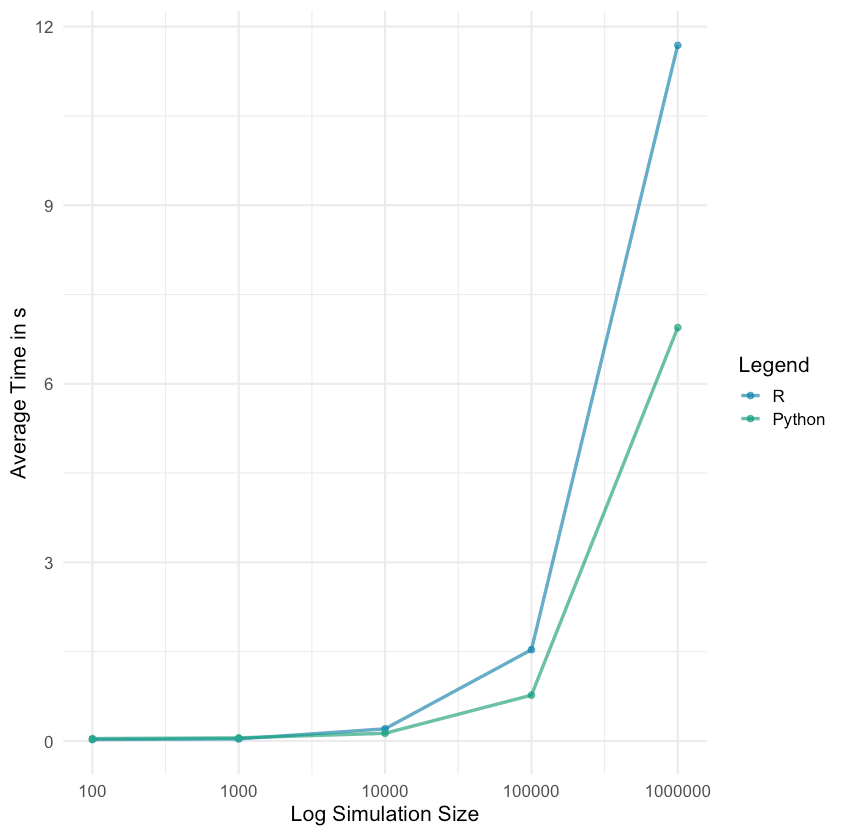
For other speed comparisons, I recommend the following STATWORX blog posts: pandas vs. data.table and pandas vs. data.table part 2. In these posts, the focus was laid on data manipulation.
The Standard in Deep Learning
If you are particularly interested in deep learning, I recommend Python to you. Most popular deep learning libraries were written or are designed to be used with Python.
Deep learning is also possible with R, but the R deep learning community is much smaller. Implementations like Keras and TensorFlow can be called in R but are run in Python in the background. Furthermore, the packages do not provide full flexibility for the users, e.g., not all TensorFlow functions are available.
A Survey in the Community
As aspiring data scientists, Kaggle is an essential platform for you. There you can participate in exciting machine learning competitions, experiment for yourself, and learn from the experiences of the community.
In 2018, Kaggle conducted a Machine Learning & Data Science Survey. The poll was online for two weeks and received a total of 23,859 replies. From the results of this survey, I have created different plots to get some insights regarding my blog topic. The code for the individual plots is publicly available on Github.
Excursion: Python & R compared to other languages
Before we jump to R and Python, let’s see how they compare to other programming languages. Each respondent indicated which language she uses primarily. The plot below aggregates by language, and the result is: Most of the participants use Python! Followed by R in second place. In this survey, we do not distinguish between fields of work, which is why Python, the general-purpose programming language, is probably so prominent.
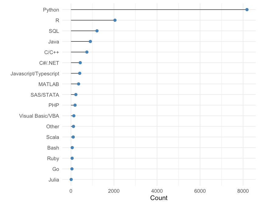
The results between R & Python
In a direct comparison between R and Python, you can see that many R users also use Python. Whereas Python users often work exclusively with Python.
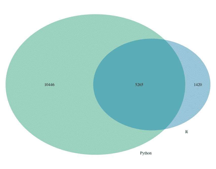
Comparing the use of languages by field reveals a clear dominance of Python. In all fields, except for statisticians, the majority uses Python.

Participants were also asked: What language do you recommend for beginners to learn first? The answers to the question are shown in the table below.
| Sprache | Empfehlung | Nutzer | Differenz |
|---|---|---|---|
| Python | 14.181 | 8.180 | 6.001 |
| R | 2.342 | 2.046 | 296 |
| SQL | 914 | 1.211 | -297 |
| C++ | 339 | 739 | -400 |
| Matlab | 256 | 355 | -99 |
| Java | 184 | 903 | -719 |
| Scala | 74 | 106 | -32 |
| Javascript | 72 | 408 | -336 |
| SAS | 69 | 228 | -159 |
| VBA | 38 | 135 | -97 |
| Go | 26 | 46 | -20 |
| Other | 161 | 117 | 44 |
When the number of recommendations and the number of users are compared, you can see that R and Python are the only languages that have a positive difference.
Again, Python (14.181) is well ahead of R (2.342).
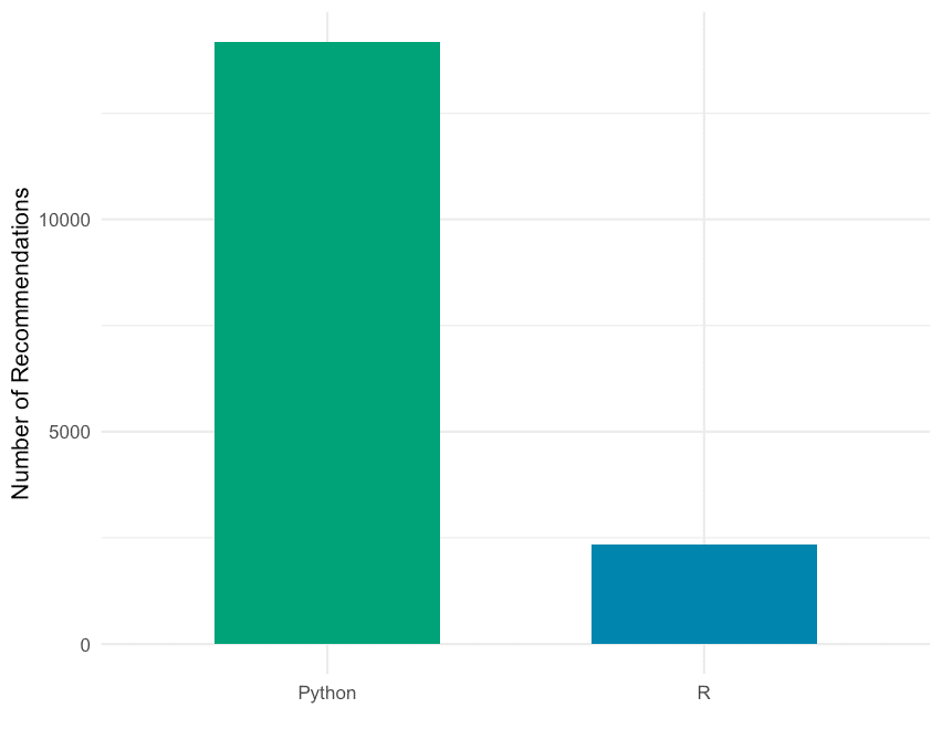
Conclusion
Beforehand: both languages are very powerful. Therefore you can not make a wrong choice! The choice of language depends on what kind of project you want to tackle.
As a universal programming language, Python is suitable for a variety of applications. Which is why I generally recommend starting with Python. But if statistical analysis or data visualization is paramount in your projects, R has an advantage over Python.
As already mentioned, both languages have their advantages and disadvantages. As an advanced data scientist, you should ideally master both languages.
I hope this post gives you an idea of what the differences are between R and Python and helps you make the right choice for yourself. Since I could not go into much depth with arguments for my preferences in this blog post – you are very welcome to shoot me an e-mail, if you have any further questions regarding the topic.
Happy Coding!
If you’re interested in training, feel free to check out our course Catalogs for R and Python at STATWORX Academy.
References
- https://cran.r-project.org/
- https://www.python.org/
- https://pipenv.readthedocs.io/en/latest/
- https://conda.io/en/latest/
- https://github.com/scikit-learn/scikit-learn/issues/6738
- https://www.rstudio.com/
- https://www.springer.com/us/book/9780387245447
- http://wiki.c2.com/?PythonPhilosophy
- https://www.kaggle.com
- https://www.statworx.com/ai-academy/
Intro
Information is everywhere online. Unfortunately, some of it is hard to access programmatically. While many websites offer an API, they are often expensive or have very strict rate limits, even if you’re working on an open-source and/or non-commercial project or product.
That’s where web scraping can come into play. Wikipedia defines web scraping as follows:
Web scraping, web harvesting, or web data extraction data scraping used for extracting data from websites. Web scraping software may access the World Wide Web directly using the Hypertext Transfer Protocol [HTTP], or through a web browser.
“Web scraping” wikipedia.org
In practice, web scraping encompasses any method allowing a programmer to access the content of a website programmatically, and thus, (semi-) automatically.
Here are three approaches (i.e. Python libraries) for web scraping which are among the most popular:
- Sending an HTTP request, ordinarily via Requests, to a webpage and then parsing the HTML (ordinarily using BeautifulSoup) which is returned to access the desired information. Typical Use Case: Standard web scraping problem, refer to the case study.
- Using tools ordinarily used for automated software testing, primarily Selenium, to access a websites‘ content programmatically. Typical Use Case: Websites which use Javascript or are otherwise not directly accessible through HTML.
- Scrapy, which can be thought of as more of a general web scraping framework, which can be used to build spiders and scrape data from various websites whilst minimizing repetition. Typical Use Case: Scraping Amazon Reviews.
While you could scrape data using any other programming language as well, Python is commonly used due to its ease of syntax as well as the large variety of libraries available for scraping purposes in Python.
After this short intro, this post will move on to some web scraping ethics, followed by some general information on the libraries which will be used in this post. Lastly, everything we have learned so far will be applied to a case study in which we will acquire the data of all companies in the portfolio of Sequoia Capital, one of the most well-known VC firms in the US. After checking their website and their robots.txt, scraping Sequoia’s portfolio seems to be allowed; refer to the section on robots.txt and the case study for details on how I went about determining this.
In the scope of this blog post, we will only be able to have a look at one of the three methods above. Since the standard combination of Requests + BeautifulSoup is generally the most flexible and easiest to pick up, we will give it a go in this post. Note that the tools above are not mutually exclusive; you might, for example, get some HTML text with Scrapy or Selenium and then parse it with BeautifulSoup.
Web Scraping Ethics
One factor that is extremely relevant when conducting web scraping is ethics and legality. I’m not a lawyer, and specific laws tend to vary considerably by geography anyway, but in general web scraping tends to fall into a grey area, meaning it is usually not strictly prohibited, but also not generally legal (i.e. not legal under all circumstances). It tends to depend on the specific data you are scraping.
In general, websites may ban your IP address anytime you are scraping something they don’t want you to scrape. We here at STATWORX don’t condone any illegal activity and encourage you to always check explicitly when you’re not sure if it’s okay to scrape something. For that, the following section will come in handy.
Understanding robots.txt
The robot exclusion standard is a protocol which is read explicitly by web crawlers (such as the ones used by big search engines, i.e. mostly Google) and tells them which parts of a website may be indexed by the crawler and which may not. In general, crawlers or scrapers aren’t forced to follow the limitations set forth in a robots.txt, but it would be highly unethical (and potentially illegal) to not do so.
The following shows an example robots.txt file taken from Hackernews, a social newsfeed run by YCombinator which is popular with many people in startups.
The Hackernews robots.txt specifies that all user agents (thus the * wildcard) may access all URLs, except the URLs that are explicitly disallowed. Because only certain URLs are disallowed, this implicitly allows everything else. An alternative would be to exclude everything and then explicitly specify only certain URLs which can be accessed by crawlers or other bots.
Also, notice the crawl delay of 30 seconds which means that each bot should only send one request every 30 seconds. It is good practice, in general, to let your crawler or scraper sleep in regular (rather large) intervals since too many requests can bring down sites down, even when they come from human users.
When looking at the robots.txt of Hackernews, it is also quite logical why they disallowed some specific URLs: They don’t want bots to pose as users by for example submitting threads, voting or replying. Anything else (e.g. scraping threads and their contents) is fair game, as long as you respect the crawl delay. This makes sense when you consider the mission of Hackernews, which is mostly to disseminate information. Incidentally, they also offer an API that is quite easy to use, so if you really needed information from HN, you would just use their API.
Refer to the Gist below for the robots.txt of Google, which is (obviously) much more restrictive than that of Hackernews. Check it out for yourself, since it is much longer than shown below, but essentially, no bots are allowed to perform a search on Google, specified on the first two lines. Only certain parts of a search are allowed, such as „about“ and „static“. If there is a general URL which is disallowed, it is overwritten if a more specific URL is allowed (e.g. the disallowing of /search is overridden by the more specific allowing of /search/about).
Moving on, we will take a look at the specific Python packages which will be used in the scope of this case study, namely Requests and BeautifulSoup.
Requests
Requests is a Python library used to easily make HTTP requests. Generally, Requests has two main use cases, making requests to an API and getting raw HTML content from websites (i.e., scraping).
Whenever you send any type of request, you should always check the status code (especially when scraping), to make sure your request was served successfully. You can find a useful overview of status codes here. Ideally, you want your status code to be 200 (meaning your request was successful). The status code can also tell you why your request was not served, for example, that you sent too many requests (status code 429) or the infamous not found (status code 404).
Use Case 1: API Requests
The Gist above shows a basic API request directed to the NYT API. If you want to replicate this request on your own machine, you have to first create an account at the NYT Dev page and then assign the key you receive to the KEY constant.
The data you receive from a REST API will be in JSON format, which is represented in Python as a dict data structure. Therefore, you will still have to „parse“ this data a bit before you actually have it in a table format which can be represented in e.g. a CSV file, i.e. you have to select which data is relevant for you.
Use Case 2: Scraping
The following lines request the HTML of Wikipedia’s page on web scraping. The status code attribute of the Response object contains the status code related to the request.
After executing these lines, you still only have the raw HTML with all tags included. This is usually not very useful, since most of the time when scraping with Requests, we are looking for specific information and text only, as human readers are not interested in HTML tags or other markups. This is where BeautifulSoup comes in.
BeautifulSoup
BeautifulSoup is a Python library used for parsing documents (i.e. mostly HTML or XML files). Using Requests to obtain the HTML of a page and then parsing whichever information you are looking for with BeautifulSoup from the raw HTML is the quasi-standard web scraping „stack“ commonly used by Python programmers for easy-ish tasks.
Going back to the Gist above, parsing the raw HTML returned by Wikipedia for the web scraping site would look similar to the below.
In this case, BeautifulSoup extracts all headlines, i.e. all headlines in the Contents section at the top of the page. Try it out for yourself!
As you can see below, you can easily find the class attribute of an HTML element using the inspector of any web browser.
Figure 1: Finding HTML elements on Wikipedia using the Chrome inspector.
This kind of matching is (in my opinion), one of the easiest ways to use BeautifulSoup: You simply specify the HTML tag (in this case, span) and another attribute of the content which you want to find (in this case, this other attribute is class). This allows you to match arbitrary sections of almost any webpage. For more complicated matches, you can also use regular expressions (REGEX).
Once you have the elements, from which you would like to extract the text, you can access the text by scraping their text attribute.
Inspector
As a short interlude, it’s important to give a brief introduction to the Dev tools in Chrome (they are available in any browser, I just chose to use Chrome), which allows you to use the inspector, that gives you access to a websites HTML and also lets you copy attributes such as the XPath and CSS selector. All of these can be helpful or even necessary in the scraping process (especially when using Selenium). The workflow in the case study should give you a basic idea of how to work with the Inspector. For more detailed information on the Inspector, the official Google website linked above contains plenty of information.
Figure 2 shows the basic interface of the Inspector in Chrome.
Figure 2: Chrome Inspector on Wikipedia.
Sequoia Capital Case Study
I actually first wanted to do this case study with the New York Times, since they have an API and thus the results received from the API could have been compared to the results from scraping. Unfortunately, most news organizations have very restrictive robots.txt, specifically not permitting searching for articles. Therefore, I decided to scrape the portfolio of one of the big VC firms in the US, Sequoia, since their robots.txt is permissive and I also think that startups and the venture capital scene are very interesting in general.
Robots.txt
First, let’s have a look at Sequoia’s robots.txt:
Luckily, they permit access of various kinds – except three URLs, which is fine for our purposes. We will still build in a crawl delay of 15-30 seconds between each request.
Next, let’s scope out the actual data which we are trying to scrape. We are interested in the portfolio of Sequoia, so https://www.sequoiacap.com/companies/ is the URL we are after.
Figure 3: Sequoia’s portfolio.
The companies are nicely laid out in a grid, making them pretty easy to scrape. Upon clicking, the page shows the details of each company. Also, notice how the URL changes in Figure 4 when clicking on a company! This is important for Requests especially.
Figure 4: Detail page on one of Sequoia’s portfolio companies.
Let’s aim for collecting the following basic information on each company and outputting them as a CSV file:
- Name of the company
- URL of the company
- Description
- Milestones
- Team
- Partner
If any of this information is not available for a company, we will simply append the string “NA” instead.
Time to start inspecting!
Scraping Process
Company Name
Upon inspecting the grid it looks like the information on each company is contained within a div tag with the class companies _company js-company. Thus we should just be able to look for this combination with BeautifulSoup.
Figure 5: Grid structure of each company.
This still leaves us with all the other information missing though, meaning we have to somehow access the detail page of each company. Notice how in Figure 5 above, each company div has an attribute called data-url. For 100 Thieves, for example, onclick has the value /companies/100-thieves/. That’s just what we need!
Now, all we have to do is to append this data-URL attribute for each company to the base URL (which is just https://www.sequoiacap.com/) and now we can send yet another request to access the detail page of each company.
So let’s write some code to first get the company name and then send another request to the detail page of each company: I will write code interspersed with text here. For a full script, check my Github.
First of all, we take care of all the imports and set up any variables we might need. We also send our first request to the base URL which contains the grid with all companies and instantiates a BeautifulSoup parser.
After we have taken care of basic bookkeeping and setup the dictionary in which we want to scrape the data, we can start working on the actual scraping, first parsing the class shown in Figure 5. As you can see in Figure 5, once we have selected the div tag with the matching class, we have to go to its first div child and then select its text, which then contains the name of the company.
On the detail page, we have basically everything we wanted. Since we already have the name of the company, all we still need are URL, description, milestones, team and the respective partner from Sequoia.
Company URL
For the URL, we should just be able to find elements by their class and then select the first element, since it seems like the website is always the first social link. You can see the inspector view in Figure 6.
But wait – what if there are no social links or the company website is not provided? In the case that the website is not provided, but a social media page is, we will simply consider this social media link the company’s de facto website. If there are no social links provided at all, we have to append an NA. This is why we check explicitly for the number of objects found because we cannot access the href attribute of a tag that doesn’t exist. An example of a company without a URL is shown in Figure 7.
Company description
As you can see in Figure 8, the p tag containing the company description does not have any additional identifiers, therefore we are forced to first access the div tag above it and then go down to the p tag containing the description and selecting its text attribute.
Milestones, Team & Partner(s)
For the last three elements, they are all located in the same structure and can thus be accessed in the same manner. We will simply match the text of their parent element and then work our way down from there.
Since the specific text elements do not have good identifying characteristics, we match the text of their parent element. Once we have the text, we go up two levels, by using the parent attribute. This brings us to the div tag belonging to this specific category (e.g. Milestones or Team). Now all that is left to do is go down to the ul tag containing the actual text we are interested in and getting its text.
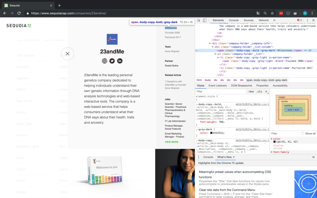
One issue with using text match is the fact that only exact matches are found. This matters in cases where the string you are looking for might differ slightly between pages. As you can see in Figure 10, this applies to our case study here for the text Partner. If a company has more than one Sequoia partner assigned to it, the string is “Partners” instead of “Partner”. Therefore we use a REGEX when searching for the partner element to get around this.
Last but not least, it is not guaranteed that all the elements we want (i.e. Milestones, Team, and Partner) are in fact available for each company. Thus before actually selecting the element, we first find all elements matching the string and then check the length. If there are no matching elements, we append NA, otherwise, we get the requisite information.
For a partner, there is always one element, thus we assume no partner information is available if there are one or fewer elements. I believe the reason that one element matching partner always shows up is the “Filter by Partner” option shown in Figure 11. As you can see, scraping often requires some iterating to find some potential issues with your script.
Writing to disk
To wrap up, we append all the information corresponding to a company to the list it belongs to within our dictionary. Then we convert this dictionary into a pandas DataFrame before writing it to disk.
Success! We just collected all of Seqouia’s portfolio companies and information on them.
* Well, all on their website at least, I believe they have their own respective sites for e.g. India and Israel.
Let’s have a look at the data we just scraped:
Looks good! We collected 506 companies in total and the data quality looks really good as well. The only thing I noticed is that some companies have a social link but it does not actually go anywhere. Refer to Figure 12 for an example of this with Pixelworks. The issue is that Pixelworks has a social link but this social link does not actually contain a URL (the href target is blank) and simply links back to the Sequoia portfolio.
I have added code in the script to replace the blanks with NAs but have left the data as is above to illustrate this point.
Conclusion
With this blog post, I wanted to give you a decent introduction to web scraping in general and specifically using Requests & BeautifulSoup. Now go use it in the wild by scraping some data that can be of use to you or someone you know! But always make sure to read and respect both the robots.txt and the terms and conditions of whichever page you are scraping.
Furthermore, you can check out resources and tutorials on some of the other methods shown above on their official websites, such as Scrapy and Selenium. You should also challenge yourself by scraping some more dynamic sites which you can not scrape using only Requests.
If you have any questions, found a bug or just feel like chatting about all things Python and scraping, feel free to contact me at david.wissel@statworx.com.