At statworx, we are constantly exploring new ideas and possibilities in the field of artificial intelligence. Recent months have been marked by generative models, particularly those developed by OpenAI (e.g., ChatGPT, DALL-E 2) but also open-source projects like Stable Diffusion. ChatGPT is a text-to-text model while DALL-E 2 and Stable Diffusion are text-to-image models, which create impressive images based on a short text description provided by the user. During the evaluation of those research trends, we discovered a great way to use our GPU to allow the statcrew to generate their own digital avatars.
The technology behind text-to-image generator Stable Diffusion
But first, let’s dive into the background of our work. Text-to-image generators, such as DALL-E 2 and Stable Diffusion, are based on diffusion architectures of artificial neural networks. It often takes months to train them on a vast amount of data from the internet, and this is only possible with supercomputers. However, even after training, the OpenAI models still require a supercomputer to generate new images, as their size exceeds the capacity of personal computers. OpenAI has made their models available through interfaces (https://openai.com/product#made-for-developers), but the model weights themselves have not been publicly released.
Stable Diffusion, on the other hand, was developed as a text-to-image generator but has a size that allows it to be executed on a personal computer. The open-source project is a joined collaboration of several research institutes. Its public availability allows researchers and developers to adapt the trained model for their own purposes by fine-tuning. Stable Diffusion is small enough to be executed on a personal computer, but fine-tuning it is significantly faster on a workstation (like ours provided by HP with two NVIDIA RTX8000 GPUs). Although it is significantly smaller than, for example, DALL-E2, the quality of the generated images is still outstanding.
All these models are controlled using prompts, which are text inputs that describe the image to be generated. Those text inputs are named prompts. For artificial intelligence, text is not natively understandable, because all these algorithms are based on mathematical operations which cannot be applied to text directly. Therefore, a common method is to generate what is known as an embedding, which means converting text into mathematical vectors. The understanding of text comes from the training of the translation model from text to embeddings. The high dimensional embedding vectors are generated in a way that the distance of the vectors to each other represents the relationship of the original texts. Similar methods are also used for images, and special models are trained to perform this task.
CLIP: A hybrid model of OpenAI for image-text integration with contrastive learning approach
One such model is CLIP, a hybrid model developed by OpenAI that combines the strengths of image recognition models and language models. The basic principle of CLIP is to embed matching text and image pairs. Those embedding vectors of the texts and images are calculated so that the distance of the vector representations of the matching pairs is minimized. A distinctive feature of CLIP is that it is trained using a contrastive learning approach, in which two different inputs are compared to each other, and the similarity between them is maximized while the similarity of non-matching pairs is minimized in the same run. This allows the model to learn more robust and transferable representations of images and texts, resulting in improved performance across a variety of tasks.
Customize image generation through Textual Inversion
With CLIP as a preprocessing step of the Stable Diffusion pipeline that creates the embeddings of the user prompts, it opens a powerful and efficient opportunity to teach the model new objects or styles. This fine-tuning is called textual inversion. Figure 1 shows this training process. With a minimum of three images of an object or style and a unique text identifier, Stable Diffusion can be steered to generate images of this specific object or style. In the first step a <tag> is chosen that aims to represent the object. In this case the object is Johannes, and a few pictures of Johannes are provided. In each training step one random image is chosen from the pictures. Further, a more explainable prompt like a “rendering of <tag>” is provided and in each training step one of those prompts is randomly chosen. The part <tag> is exchanged by the defined tag (in this case <Johannes>). With textual inversion the model’s dictionary is expanded and after sufficient training steps the new fine-tuned model can be plugged into the Stable Diffusion pipeline. This leads to a new image of Johannes whenever the tag <Johannes> is part of the user prompt. Styles and other objects can be added to the generated image, depending on the prompt.
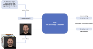
Figure 1: Fine-tuning CLIP with textual inversion.
This is what it looks like when we create AI-generated avatars of our #statcrew
At statworx, we did so with all interested colleagues which enabled them to set their digital avatars in the most diverse contexts. With the HP workstation at hand, we could use the integrated NVIDIA RTX8000 GPUs and hereby reduce the training time by a factor of 15 compared to a desktop CPU. As you can see from the examples below, the statcrew enjoyed it to generate a bunch of images in the most different situations. The following pictures show a few selected portraits of your most trusted AI consultants. 🙂
![]()
Prompts from top left to bottom right:
- <Andreas> looks a lot like christmas, santa claus, snow
- Robot <Paul>
- <Markus> as funko, trending on artstation, concept art, <Markus>, funko, digital art, box (, superman / batman / mario, nintendo, super mario)
- <Johannes> is very thankful, art, 8k, trending on artstation, vinyl·
- <Markus> riding a unicorn, digital art, trending on artstation, unicorn, (<Markus> / oil paiting)·
- <Max> in the new super hero movie, movie poster, 4k, huge explosions in the background, everyone is literally dying expect for him
- a blonde emoji that looks like <Alex>
- harry potter, hermione granger from harry potter, portrait of <Sarah>, concept art, highly detailed
Stable Diffusion together with Textual Inversion represent exciting developments in the field of artificial intelligence. They offer new possibilities for creating unique and personalized avatars but it’s also applicable to styles. By continuing to explore these and other AI models, we can push the boundaries of what is possible and create new and innovative solutions to real-world problems. Stay tuned!
Image Source: Adobe Stock 546181349
What to expect:
The tremendous development of language models like ChatGPT has exceeded our expectations. Enterprises should therefore understand how they can benefit from these advances.
In our workshop “ChatGPT for Leaders”, which is geared towards executive positions, we provide compact and immediately applicable expertise, offer the opportunity to discuss the opportunities and risks of ChatGPT with other executives and industry experts, and use use cases to show how you can automate processes in your company. Look forward to exciting presentations, including from Timo Klimmer, Global Blackbelt – AI, at Microsoft and Fabian Müller, COO at statworx.
More information and a registration option is available here: ChatGPT for Leaders Workshop
It’s no secret that the latest language models like ChatGPT have far exceeded our wildest expectations. It’s impressive and even somewhat eerie to think that a language model possesses both a broad knowledge base and the ability to convincingly answer (almost) any question. Just a few hours after the release of this model, speculation began about which fields of activity could be enriched or even replaced by these models, which use cases can be implemented, and which of the many new start-up ideas arising from ChatGPT will prevail.
There is no doubt that the continuous development of artificial intelligence is gaining momentum. While ChatGPT is based on a third-generation model, a “GPT-4” is already on the horizon, and competing products are also waiting for their big moment.
As decision-makers in a company, it is now important to understand how these advancements can actually be used to add value. In this blog post, we will focus on the background instead of the hype, provide examples of specific use cases in corporate communication, and particularly explain how the implementation of these AI systems can be successful.
What is ChatGPT?
If you ask ChatGPT this question, you will receive the following answer:
“ChatGPT is a large language model trained by OpenAI to understand and generate natural language. It uses deep learning and artificial intelligence technology to conduct human-like conversations with users.”
ChatGPT is the latest representative from a class of AI systems that process human language (i.e. texts). This is called “Natural Language Processing”, or NLP for short. It is the product of a whole chain of innovations that began in 2017 with a new AI architecture. In the following years, the first AI models were developed based on this architecture that reached human-level language understanding. In the last two years, the models learned to write and even have whole conversations with the user using ChatGPT. Compared to other models, ChatGPT stands out for generating credible and appropriate responses to user requests.
In addition to ChatGPT, there are now many other language models in different forms: open source, proprietary, with dialog options or other capabilities. It quickly became apparent that these capabilities continued to grow with larger models and more (especially high-quality) data. Unlike perhaps originally expected, there seems to be no upper limit. On the contrary, the larger the models, the more capabilities they gain!
These linguistic abilities and the versatility of ChatGPT are amazing, but the use of such large models is not exactly resource-friendly. Large models like ChatGPT are operated by external providers who charge for each request to the model. In addition, every request to larger models not only generates more costs but also consumes more electricity and thus affects the environment.
For example, most chat requests from customers do not require comprehensive knowledge of world history or the ability to give amusing answers to every question. Instead, existing chatbot services tailored to business data can deliver concise and accurate answers at a fraction of the cost.
Modern Language Models in Business Applications
Despite the potential environmental and financial costs associated with large language models like ChatGPT, many decision-makers still want to invest in them. The reason lies in their integration into organizational processes. Large generative models like ChatGPT enable us to use AI in every phase of business interaction: incoming customer communication, communication planning and organization, outgoing customer communication and interaction execution, and finally, process analysis and improvement.
In the following, we will explain in detail how AI can optimize and streamline these communication processes. It quickly becomes clear that it is not just a matter of applying a single advanced AI model. Instead, it becomes apparent that only a combination of multiple models can effectively address the challenges and deliver the desired economic benefits in all phases of interaction.
For example, AI systems are becoming increasingly relevant in communication with suppliers or other stakeholders. However, to illustrate the revolutionary impact of new AI models more concretely, let us consider the type of interaction that is vital for every company: communication with the customer.
Use Case 1: Incoming Customer Communication with AI.
Challenge
Customer inquiries are received through various channels (emails, contact forms on the website, apps, etc.) and initiate internal processes and workflows within the CRM system. Unfortunately, the process is often inefficient and leads to delays and increased costs due to inquiries being misdirected or landing in a single central inbox. Existing CRM systems are often not fully integrated into organizational workflows and require additional internal processes based on organic routines or organizational knowledge of a small number of employees. This reduces efficiency and leads to poor customer satisfaction and high costs.
Solution
Customer communication can be a challenge for businesses, but AI systems can help automate and improve it. With the help of AI, the planning, initiation, and routing of customer interactions can be made more effective. The system can automatically analyze content and information and decide how best to handle the interaction based on appropriate escalation levels. Modern CRM systems are already able to process standard inquiries using low-cost chatbots or response templates. But if the AI recognizes that a more complex inquiry is present, it can activate an AI agent like ChatGPT or a customer service representative to take over the communication.
With today’s advances in the NLP field, an AI system can do much more. Relevant information can be extracted from customer inquiries and forwarded to the appropriate people in the company. For example, a key account manager can be the recipient of the customer message while a technical team is informed with the necessary details. In this way, more complex scenarios, the organization of support, the distribution of workloads, and the notification of teams about coordination needs can be handled. These processes are not manually defined but learned by the AI system.
More details such as technical architecture, vendors, pros and cons of models, requirements and timelines can be found in the following download:
The implementation of an integrated system can increase the efficiency of a company, reduce delays and errors, and ultimately lead to higher revenue and profit.
Use Case 2: Outgoing Customer Communication with AI.
Challenge
Customers expect their inquiries to be promptly, transparently, and precisely answered. A delayed or incorrect response, a lack of information, or uncoordinated communication between different departments are breaches of trust that can have a negative long-term effect on customer relationships.
Unfortunately, negative experiences are commonplace in many companies. This is often because existing solutions’ chatbots use standard answers and templates and are only rarely able to fully and conclusively answer customer inquiries. In contrast, advanced AI agents like ChatGPT have higher communication capabilities that enable smooth customer communication.
When the request does reach the right customer service employees, new challenges arise. Missing information regularly leads to sequential requests between departments, resulting in delays. Once processes, intentionally or unintentionally, run in parallel, there is a risk of incoherent communication with the customer. Ultimately, both internally and externally, transparency is lacking.
Solution
AI systems can support companies in all areas. Advanced models like ChatGPT have the necessary linguistic abilities to fully process many customer inquiries. They can communicate with customers and at the same time ask internal requests. This makes customers no longer feel brushed off by a chatbot. The technical innovations of the past year allow AI agents to answer requests not only faster but also more accurately. This relieves the customer service and internal process participants and ultimately leads to higher customer satisfaction.
AI models can also support human employees in communication. As mentioned at the beginning, there is often simply a lack of accurate and precise information available in the shortest possible time. Companies are striving to break down information silos to make access to relevant information easier. However, this can lead to longer processing times in customer service, as the necessary information must first be collected. An essential problem is that information can be presented in various forms, such as text, tabular data, in databases, or even in the form of structures like previous dialogue chains.
Modern AI systems can handle unstructured and multimodal information sources. Retrieval systems connect customer requests to various information sources. The additional use of generative models like GPT-3 then allows the found information to be efficiently synthesized into understandable text. Individual “Wikipedia articles” can be generated for each customer request. Alternatively, the customer service employee can ask a chatbot for the necessary information, which is immediately and understandably provided.
It is evident that an integrated AI system not only relieves customer service but also other technical departments. This type of system has the potential to increase efficiency throughout the company.
Use Case 3: Analysis of communication with AI
Challenge
Robust and efficient processes do not arise on their own, but through continuous feedback and constant improvements. The use of AI systems does not change this principle. An organization needs a process of continuous improvement to ensure efficient internal communication, effectively manage delays in customer service, and conduct result-oriented sales conversations.
However, in outward dialogue, companies face a problem: language is a black box. Words have unparalleled information density precisely because their use is deeply rooted in context and culture. This means that companies evade classical statistical-causal analysis because communication nuances are difficult to quantify.
Existing solutions therefore use proxy variables to measure success and conduct experiments. While overarching KPIs such as satisfaction rankings can be extracted, they must be obtained from the customer and often have little meaning. At the same time, it is often unclear what can be specifically changed in customer communication to modify these KPIs. It is difficult to analyze interactions in detail, identify dimensions and levers, and ultimately optimize them. The vast majority of what customers want to reveal about themselves immediately exists in text and language and evades analysis. This problem arises both with the use of AI assistance systems and with customer service representatives.
Solution
While modern language models have received much attention due to their generative capabilities, their analytical capabilities have also made enormous strides. The ability of AI models to respond to customer inquiries demonstrates an advanced understanding of language, which is essential for improving integrated AI systems. Another application is the analysis of conversations, including the analysis of customers and their own employees or AI assistants.
By using artificial intelligence, customers can be more precisely segmented by analyzing their communication in detail. Significant themes are captured and customer opinions are evaluated. Semantic networks can be used to identify which associations different customer groups have with products. In addition, generative models are used to identify desires, ideas, or opinions from a wealth of customer voices. Imagine being able to personally go through all customer communication in detail instead of having to rely on synthetic KPIs – that’s exactly what AI models make possible.
Of course, AI systems also offer the ability to analyze and optimize their own processes. AI-supported dialogue analysis is a promising area of application that is currently being intensively researched. This technology enables, for example, the examination of sales conversations with regard to successful closures. Breaking points in the conversation, changes in mood and topics are analyzed to identify the optimal course of a conversation. This type of feedback is extremely valuable not only for AI assistants but also for employees because it can even be played during a conversation.
In summary, the use of AI systems improves the breadth, depth, and speed of feedback processes. This allows the organization to be agile in responding to trends, desires, and customer opinions and to further optimize internal processes.
More details such as technical architecture, vendors, pros and cons of models, requirements and timelines can be found in the following download:
Obstacles to consider when implementing AI systems
The application of AI systems has the potential to fundamentally revolutionize communication with customers. Similar potential can also be demonstrated in other areas, such as procurement and knowledge management, which are discussed in more detail in the accompanying materials.
However, it is clear that even the most advanced AI models are not yet ready for deployment in isolation. To move from experimentation to effective implementation, it takes experience, good judgment, and a well-coordinated system of AI models.
The integration of language models is even more important than the models themselves. Since language models act as the interface between computers and humans, they must meet specific requirements. In particular, systems that intervene in work processes must learn from the established structures of the company. As interface technology, aspects such as fairness, impartiality, and fact-checking must be integrated into the system. In addition, the entire system needs a direct intervention capability for employees to identify errors and realign the AI models if necessary. This “active learning” is not yet standard, but it can make the difference between theoretical and practical efficiency.
The use of multiple models that run both on-site and directly from external providers presents new demands on the infrastructure. It is also important to consider that essential information transfer is not possible without careful treatment of personal data, especially when critical company information must be included. As described earlier, there are now many language models with different capabilities. Therefore, the solution’s architecture and models must be selected and combined according to the requirements.
Finally, there is the question of whether to rely on solution providers or develop your own (partial) models. Currently, there is no standard solution that meets all requirements, despite some marketing claims. Depending on the application, there are providers of cost-effective partial solutions. Making a decision requires knowledge of these providers, their solutions, and their limitations.
Conclusion
In summary, it can be stated that the use of AI systems in customer communication can improve and automate processes. A central objective for companies should be the optimization and streamlining of their communication processes. AI systems can support this by making the planning, initiation, and forwarding of customer interactions more effective and by either activating a chatbot like ChatGPT or a customer service representative for more complex inquiries. By combining different models in a targeted manner, meaningful problem-solving can be achieved in all phases of interaction, generating the desired economic benefits.
More details such as technical architecture, vendors, pros and cons of models, requirements and timelines can be found in the following download:
It’s Christmas time at statworx: Christmas songs are playing during the lunch break, the office is festively decorated and the Christmas party was already a great success. But statworx wouldn’t be a consulting and development company in the area of data science, machine learning and AI if we didn’t bring our expertise and passion to our Christmas preparations.
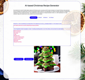
Surrounded by the smell of freshly baked cookies and Christmas punch, we came up with the idea of developing an AI-based Christmas recipe generator that can complete and visualize texts of any kind using OpenAI models. With GPT-3, the description of a recipe is enough to generate a complete list of ingredients as well as cooking instructions. Afterwards, the complete text is passed as an image description to DALL-E 2, which visualizes it in a high-resolution image. Of course, the application of both models goes far beyond the entertainment factor in day-to-day work, but we believe that a playful get-to-know-you session with the models over cookies and mulled wine is the ideal approach.
Before we get creative together and test the Christmas recipe generator, we will first take a brief look at the models behind it in this blog post.
The leaves are falling but AI is blossoming with the help of GPT-3
The pace of development of large-language models and text-to-image models over the past two years has been breathtaking and swept all of our employees along with it. From avatars and internal memes to synthetic data on projects, not only the quality of the results has changed, but also the handling of the models. Where once there was performant code, statistical analysis, and lots of Greek letters floating around, now the operation of some models almost takes the form of an exchange or interaction. So-called prompts are created by means of texts or keyword prompts.
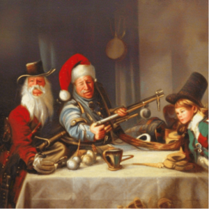
Fig. 1: Fancy a Christmas punch with a shot? The starting point for this image was the prompt “A rifle pointed at a Christmas mug”. By a lot of trial and error and mostly unexpectedly detailed prompts with many keywords, the results can be strongly influenced.
This form of interaction is partially due to the GPT-3 language model, which is based on a Deep Learning model. The arrival of this revolutionary language model not only represented a turning point for the research field of language modeling (NLP), but incidentally heralded a paradigm shift in AI development: prompt engineering.
While many areas of machine learning remain unaffected, for other areas it even meant the biggest breakthrough since the use of neural networks. As before, probability distributions are learned, target variables are predicted, or embeddings are used, i.e. a kind of compressed neuronal intermediate product, which are optimized for further processing and information content. For other use cases, mostly of a creative nature, it is now sufficient to specify the desired result in natural language and match it to the behavior of the models. More on prompt engineering can be found in this blog post.
In general, the ability of the so-called Transformer models to capture a sentence and its words as a dynamic context is one of the most important innovations. Nevertheless, one must pay attention! Words (in this case cooking and baking ingredients) can have different meanings in different recipes. And these relationships can now be captured by the model. In our first AI cooking experiments, this was not yet the case. When rigid Word2Vec models were used, beef broth or pureed tomatoes might be recommended instead of or along with red wine. Regardless of whether it was jelly for cookies or mulled wine, as the hearty use predominated in the training data!
Christmas image generation with DALL-E 2
In our Christmas recipe generator, we use DALL-E 2 to then generate an image from the completed text. DALL-E 2 is a neural network that can generate high-resolution images based on text descriptions. There are no limitations – the images resulting from the creative word input make the impossible seem possible. However, misunderstandings often occur, as can be seen in some of the following examples.

Fig. 2: Experienced programmers will immediately recognize this: It’s not you, it’s me! Complex, pedantic, or simply logical… Programs usually show us errors or loose assumptions immediately.
Now getting acquainted with the model becomes even more important, because small changes in the prompt or certain keywords can strongly influence the result. Websites like PromptHero collect previous results including prompts (by the way, the experience values differ depending on the model) and give inspiration for high-resolution generated images.
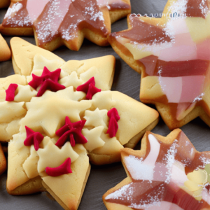
Fig. 3: We wanted to test what was possible and generated cinnamon cookies and gingerbread hawaii with pineapple and ham. The results are still off the scale of taste and dignity.
And how would the model make a coffee at the Acropolis or in a Canadian Indian summer? Or a pun(s)ch with a kick?
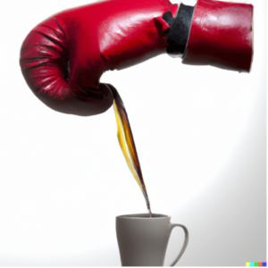
Fig. 4: Packs quite the punch.
Complex technology, informal getting to know each other
Enough theory and back to practice.
Now it’s time to test our Christmas recipe generator and have a cooking recipe recommended to you based on a recipe name and an incomplete list of desired ingredients. Creative names, descriptions and shapes are encouraged, unconventional ingredients are strictly desired and model surprising interpretations are almost pre-programmed.
Go to Christmas Recipe Generator
The GPT-3 model used for text completion is so diverse that all of Wikipedia doesn’t even make up 0.1% of the training data and there is no end in sight for possible new use cases. Just open our little WebApp to generate punch, cookie or any recipe and be amazed how far the developments in Natural Language Processing and Text-to-Image have come.
We wish you a lot of fun!
We, the members of the computer vision working group at statworx, had set ourselves the goal of building more competencies in our field with the help of exciting projects. For this year’s statworx Alumni Night, which took place at the beginning of September, we came up with the idea of a greeting robot that would welcome the arriving employees and alumni of our company with a personal message. To realize this project, we planned to develop a facial recognition model on a Waveshare JetBot. The Jetbot is powered by an NVIDIA Jetson Nano, a small, powerful computer with a 128-core GPU for fast execution of advanced AI algorithms. Many popular AI frameworks such as Tensorflow, PyTorch, Caffe, and Keras are supported. The project seemed to be a good opportunity for both experienced and inexperienced members of our working group to build knowledge in computer vision and gain experience in robotics.
Face recognition using the JetBot required solving several interrelated problems:
- Face Detection: Where is the face located in the image?
First, the face must be located on the provided image. Only this part of the image is relevant for all subsequent steps. - Face embedding: What are the unique features of the face?
Next, unique features must be identified and encoded in an embedding that is used to distinguish it from other people. An associated challenge is for the model to learn how to deal with slopes of the face and poor lighting. Therefore, before creating the embedding, the pose of the face must be determined and corrected so that the face is centered. - Name determination: Which embedding is closest to the recognized face?
Finally, the embedding of the face must be compared with the embeddings of all the people the model already knows to determine the name of the person. - UI with welcome message
We developed a UI for the welcome message. For this, we had to create a mapping beforehand that maps the name to a welcome message. - Configuration of the JetBot
The last step was to configure the JetBot and transfer the model to the JetBot.
Training such a face recognition model is very computationally intensive, as millions of images of thousands of different people are used to obtain a powerful neural network. However, once the model is trained, it can generate embeddings for any face (known or unknown). Therefore, we were fortunately able to use existing face recognition models and only had to create embeddings from the faces of our colleagues and alumni. Nevertheless, I’ll briefly explain the training steps to give an understanding of how these face recognition models work.
We used the Python package face_recognition, which wraps the face recognition functionality of dlib to make it easier to work with. Its neural network was trained on a dataset of about 3 million images and achieved 99.38% accuracy on the Labeled Faces in the Wild (LFW) dataset, outperforming other models.
From an image to the encoded face (Face Detection)
The localization of a face on an image is done by the Histogram of Oriented Gradients (HOG) algorithm. In this process, each individual pixel of the image is compared with the pixels in the immediate vicinity and replaced by an arrow pointing in the direction in which the image becomes darker. These arrows represent the gradients and show the progression from light to dark across the entire image. To create a clearer structure, the arrows are aggregated at a higher level. The image (a) is divided into small squares of 16×16 pixels each and replaced with the arrow direction that occurs most frequently (b). Using the HOG-encoded version of the image, the image sector that is closest to a HOG-encoded face (c) can now be found. Only this part of the image is relevant for the following steps.
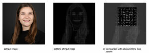
Figure 1: Turning an image to a HOG pattern
source: https://commons.wikimedia.org/wiki/File:Dlib_Learned-HOG-Detector.jpg
Making faces learnable with embeddings
For the face recognition model to be able to assign different images of a person to the same face despite some images being tilted or suffering from poor lighting, the pose of the face needs to be determined and used for projection so that the eyes and lips are always in the same position of the resulting image. This is done using the Face Landmark Estimation algorithm, which can find specific landmarks in a face using machine learning. This allows us to locate the eyes and mouth and adjust them using basic image transformations such as rotation and scaling, so that the facial features are as centered as possible.
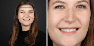
Figure 2: Face landmarks (left) and projection of the face (right)
In the next step, a neural network is used to create an embedding of the centered face image. The neural network learns meaningful embeddings by looking at three face images simultaneously within one training step: Two images of a known person and one image of another person. The neural network creates the embeddings of the three images and optimizes its weights so that the embeddings of the images of the same person are approximated and differ more with the embedding of the other person. After repeating this step millions of times for different images of different people, the neural network learns to generate representative embeddings. The network architecture of dlib‘s face recognition model is based on ResNet-34 from the paper Deep Residual Learning for Image Recognition by He et al., with fewer layers and several filters reduced by half. The generated embeddings are 128-dimensional.
Matching faces with learned embeddings in real time
Fortunately, we could use the existing model from dlib for our robot. For the model to recognize the faces of the current and former statcrew, we only had to create embeddings of everyone’s faces. For this we used the official statworx portraits and saved the resulting embedding together with each respective name. If an unknown image is then fed into the model, the face is detected, centered and turned into an embedding. The created embedding is then matched with the stored embeddings of the known people and if there is a high similarity, the name of this person is returned. If there is no similar embedding, there is no match with the knows faces. More images of a person and thus multiple embeddings per person would improve the performance of the model. However, our tests showed that our faces were recognized quite reliably even with only one image per person. After this step, we now had a good model that recognized faces in the camera in real time and displayed the associated name.
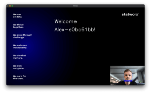
A warm welcome via a UI
Our plan was to equip the robot with a small screen or speaker so the welcome message could be seen or heard. As a starting point, we settled on connecting the robot to a monitor and building a UI to display the message. First, we developed a simple UI which displayed the welcome message in front of a background with the statworx company values and projected the camera image in the lower right corner. For each person to receive a personalized message, we had to create a json file that defined the mapping from the names to the welcome message. For unfamiliar faces, we had created the welcome message “Welcome Stranger!”. Because of the many namesakes at statworx, everyone with the name Alex also received a unique identifier:
Last hurdles before commissioning the robot
Since the model and the UI were only running locally so far, there was still the task of transferring the model to the robot with its integrated camera. Unfortunately, we found out that this was more complicated than expected. We were faced with memory problems time and again, meaning that we had to reconfigure the robot a total of three times before we could successfully deploy the model. The instructions for configuring the robot, which helped us succeed in the end, can be found here: https://jetbot.org/master/software_setup/sd_card.html. The memory problems could mostly be solved with a reboot.
The use of the welcome robot at the Alumni Night
Our welcome robot was a great success at the Alumni Night! Our guests were very surprised and happy about the personalized message.
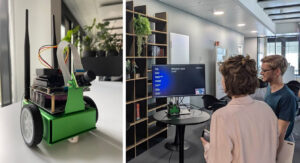
Figure 3: Welcoming guests to the statworx-Alumni-Night
The project was also a big success for the Computer Vision cluster. During the project, we learned a lot about face recognition models and all the challenges associated with them. Working with the JetBot was particularly exciting and we are already planning more projects with the robot for next year.
What to expect:
On 15.12.2022 we will host the next UAI at Villa Bethmann in Frankfurt. At the event, you can network and exchange ideas with our AI talents, AI startups and AI experts from different companies.
Our AI Hub (UAI) event series and the AI community in Frankfurt Rhine Main is growing at a rapid pace. It is incredible how much momentum UAI has built up and brought to Frankfurt in less than 6 months. Two events with over 600 guests and an AI network consisting of regional and national start-ups, corporations, AI talents and AI experts.
At this XMAS Special there will be an interesting agenda with AI experts from Miele, Levi Strauss & CO, Clark, Milch und Zucker, Women in AI & Robotics, statworx, AI Frankfurt Rhein Main e.V., Crytek and many more!
We will present our AI Hub Frankfurt project with our partners Google, Microsoft, TÜV Süd and the programme for 2023.
Here are a few interesting facts and agenda items about the UAI XMAS Special:
- You can exchange ideas and network with the AI experts
- Get to know interesting AI projects
- Get to know the crepe robot from Karlsruhe University of Applied Sciences
- The special thing: There will be delicious mulled wine from AI Gude (Gude).
Tickets for the event can be purchased here: https://pretix.eu/STATION/XMAS/
statworx, AI Frankfurt Rhein Main e.V, STATION, Wirtschaftsinitiative Frankfurt Rhein Main, Wirtschaftsförderung Frankfurt Rhein Main, Frankfurt Rhein Main GmbH, StartHubHessen, TÜV Süd have made this great UAI XMAS Special possible.
What to expect:
AI, data science, machine learning, deep learning and cybersecurity talents from FrankfurtRhineMain take note!
The AI Talent Night, a networking event with a difference, offers you the opportunity to meet other talents as well as potential employers and AI experts. But that’s not all, because a great ambience, delicious food, live music, AI visualization and 3 VIP talks by leading AI experts from the business world await you.
And the best part: Are you a talent? Then you can join us for free.
Together with our partners AI FrankfurtRheinMain e.V. and STATION HQ, we are organizing the AI Talent Night as part of the UAI conference series. Our goal is to promote AI in our region and establish an AI hub in Frankfurt.
Become a part of our AI community!
Tickets for the event can be purchased here: https://pretix.eu/STATION/UAI-Talent/
or on our website:
Car Model Classification III: Explainability of Deep Learning Models with Grad-CAM
In the of this series on car model classification, we built a model using transfer learning to classify the car model through an image of a car. In the , we showed how TensorFlow Serving can be used to deploy a TensorFlow model using the car model classifier as an example. We dedicate this third post to another essential aspect of deep learning and machine learning in general: the explainability of model predictions.
We will start with a short general introduction on the topic of explainability in machine learning. Next, we will briefly talk about popular methods that can be used to explain and interpret predictions from CNNs. We will then explain Grad-CAM, a gradient-based method, in-depth by going through an implementation step by step. Finally, we will show you the results we obtained by our Grad-CAM implementation for the car model classifier.
A Brief Introduction to Explainability in Machine Learning
For the last couple of years, explainability was always a recurring but still niche topic in machine learning. But, over the past four years, interest in this topic has started to accelerate. At least one particular reason fuelled this development: the increased number of machine learning models in production. On the one hand, this leads to a growing number of end-users who need to understand how models are making decisions. On the other hand, an increasing number of machine learning developers need to understand why (or why not) a model is functioning in a particular way.
This increasing demand in explainability led to some, both methodological and technical, noteworthy innovations in the last years:
-
– a model agnostic explanation technique that uses an interpretable local surrogate model
-
– a method inspired by game theory
-
– a method to indicate discriminative image regions used by the CNN to identify a specific category (e.g., in classification tasks)
Methods for Explaining CNN Outputs for Images
Deep neural networks and especially complex architectures like CNNs were long considered as pure black box models. As written above, this changed in recent years, and now there are various methods available to explain CNN outputs. For example, the excellent library implements a wide range of useful methods for TensorFlow 2.x. We will now briefly talk about the ideas of different approaches before turning to Grad-CAM:
Activations Visualization
This is the most straightforward visualization technique. It simply shows the output of a specific layer within the network during the forward pass. It can be helpful to get a feel for the extracted features since, during training, most of the activations tend towards zero (when using the ReLu-activation). An example for the output of the first convolutional layer of the car model classifier is shown below:

Vanilla Gradients
One can use the vanilla gradients of the predicted classes’ output for the input image to derive input pixel importances.
We can see that the highlighted region is mainly focused on the car. Compared to other methods discussed below, the discriminative region is much less confined.
Occlusion Sensitivity
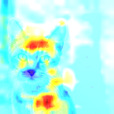
This approach computes the importance of certain parts of the input image by reevaluating the model’s prediction with different parts of the input image hidden. Parts of the image are hidden iteratively by replacing them by grey pixels. The weaker the prediction gets with a part of the image hidden, the more important this part is for the final prediction. Based on the discriminative power of the regions of the image, a heatmap can be constructed and plotted. Applying occlusion sensitivity for our car model classifier did not yield any meaningful results. Thus, we show ‘s sample image, showing the result of applying the occlusion sensitivity procedure for a cat image.
CNN Fixations
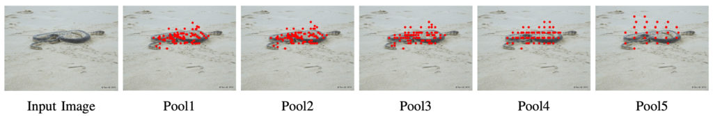
Another exciting approach called CNN Fixations was introduced in . The idea is to backtrack which neurons were significant in each layer, given the activations from the forward pass and the network weights. The neurons with large influence are referred to as fixations. This approach thus allows finding the essential regions for obtaining the result without the need for any recomputation (e.g., in the case of occlusion sensitivity above, where multiple predictions must be made).
The procedure can be described as follows: The node corresponding to the class is chosen as the fixation in the output layer. Then, the fixations for the previous layer are computed by computing which of the nodes have the most impact on the next higher level’s fixations determined in the last step. The node importance is computed by multiplying activations and weights. If you are interested in the details of the procedure, check out or the corresponding . This backtracking is done until the input image is reached, yielding a set of pixels with considerable discriminative power. An example from the paper is shown below.
CAM
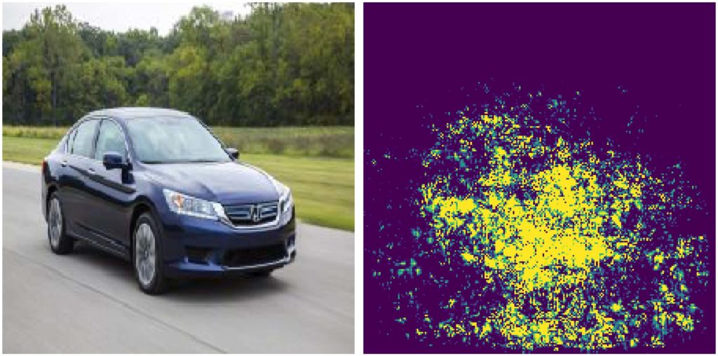
Introduced in , class activation mapping (CAM) is a procedure to find the discriminative region(s) for a CNN prediction by computing class activation maps. A significant drawback of this procedure is that it requires the network to use global average pooling (GAP) as the last step before the prediction layer. It thus is not possible to apply this approach to general CNNs. An example is shown in the figure below (taken from the ):
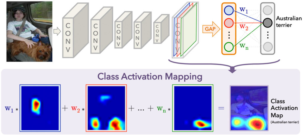
The class activation map assigns importance to every position (x, y) in the last convolutional layer by computing the linear combination of the activations, weighted by the corresponding output weights for the observed class (Australian terrier in the example above). The resulting class activation mapping is then upsampled to the size of the input image. This is depicted by the heat map above. Due to the architecture of CNNs, the activation, e.g., in the top left for any layer, is directly related to the top left of the input image. This is why we can conclude which input regions are important by only looking at the last CNN layer.
The Grad-CAM procedure we will discuss in detail below is a generalization of CAM. Grad-CAM can be applied to networks with general CNN architectures, containing multiple fully connected layers at the output.
Grad-CAM
on GitHub.
import pickle
import tensorflow as tf
import cv2
from car_classifier.modeling import TransferModel

INPUT_SHAPE = (224, 224, 3)

# Load list of targets
file = open('.../classes.pickle', 'rb')
classes = pickle.load(file)

# Load model
model = TransferModel('ResNet', INPUT_SHAPE, classes=classes)
model.load('...')

# Gradient model, takes the original input and outputs tuple with:
# - output of conv layer (in this case: conv5_block3_3_conv)
# - output of head layer (original output)
grad_model = tf.keras.models.Model([model.model.inputs],
                                   [model.model.get_layer('conv5_block3_3_conv').output,
                                    model.model.output])

# Run model and record outputs, loss, and gradients
with tf.GradientTape() as tape:
    conv_outputs, predictions = grad_model(img)
    loss = predictions[:, label_idx]

# Output of conv layer
output = conv_outputs[0]

# Gradients of loss w.r.t. conv layer
grads = tape.gradient(loss, conv_outputs)[0]

# Guided Backprop (elimination of negative values)
gate_f = tf.cast(output > 0, 'float32')
gate_r = tf.cast(grads > 0, 'float32')
guided_grads = gate_f * gate_r * grads

# Average weight of filters
weights = tf.reduce_mean(guided_grads, axis=(0, 1))

# Class activation map (cam)
# Multiply output values of conv filters (feature maps) with gradient weights
cam = np.zeros(output.shape[0: 2], dtype=np.float32)
for i, w in enumerate(weights):
    cam += w * output[:, :, i]

# Or more elegant:
# cam = tf.reduce_sum(output * weights, axis=2)

# Rescale to org image size and min-max scale
cam = cv2.resize(cam.numpy(), (224, 224))
cam = np.maximum(cam, 0)
heatmap = (cam - cam.min()) / (cam.max() - cam.min())- The first step is to load an instance of the model.
- Then, we create a new
keras.Modelinstance that has two outputs: The activations of the last CNN layer ('conv5_block3_3_conv') and the original model output. - Next, we run a forward pass for our new
grad_modelusing as input an image (img) of shape (1, 224, 224, 3), preprocessed with theresnetv2.preprocess_inputmethod. is set up and applied to record the gradients (the gradients are stored in thetapeobject). Further, the outputs of the convolutional layer (conv_outputs) and the head layer (predictions) are stored as well. Finally, we can uselabel_idxto get the loss corresponding to the label we want to find the discriminative regions for. - Using the
gradient-method, one can extract the desired gradients fromtape. In this case, we need the gradient of the loss w.r.t. the output of the convolutional layer. - In a further step, a guided backprop is applied. Only values for the gradients are kept where both the activations and the gradients are positive. This essentially means restricting attention to the activations which positively contribute to the wanted output prediction.
- The
weightsare computed by averaging the obtained guided gradients for each filter. - The class activation map
camis then computed as the weighted average of the feature map activations (output). The method containing the for loop above helps understanding what the function does in detail. A less straightforward but more efficient way to implement the CAM-computation is to usetf.reduce_meanand is shown in the commented line below the loop implementation. - Finally, the resampling (resizing) is done using OpenCV2’s
resizemethod, and the heatmap is rescaled to contain values in [0, 1] for plotting.
A version of Grad-CAM is also implemented in .
We now use the Grad-CAM implementation to interpret and explain the predictions of the TransferModelfor car model classification. We start by looking at car images taken from the front.
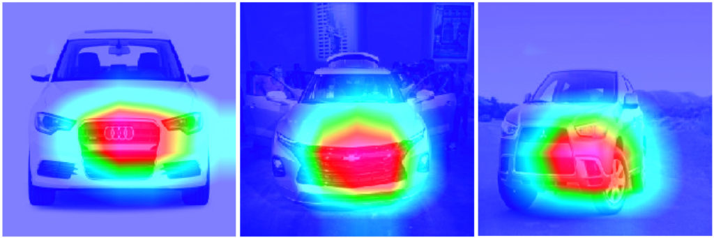
Grad-CAM for car images from the front
The red regions highlight the most important discriminative regions, the blue regions the least important. We can see that for images from the front, the CNN focuses on the car’s grille and the area containing the logo. If the car is slightly tilted, the focus is shifted more to the edge of the vehicle. This is also the case for slightly tilted images from the car’s backs, as shown in the middle image below.
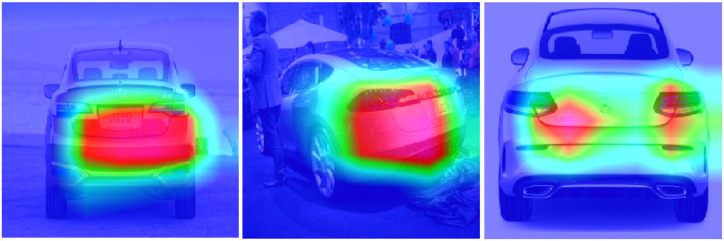
Grad-CAM for car images from the back
For car images from the back, the most crucial discriminative region is near the number plate. As mentioned above, for cars looked at from an angle, the closest corner has the highest discriminative power. A very interesting example is the Mercedes-Benz C-class on the right side, where the model not only focuses on the tail lights but also puts the highest discriminative power on the model lettering.
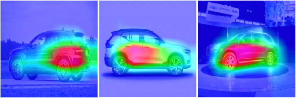
Grad-CAM for car images from the side
When looking at images from the side, we notice the discriminative region is restricted to the bottom half of the cars. Again, the angle the car image was taken from determines the shift of the region towards the front or back corner.
In general, the most important fact is that the discriminative areas are always confined to parts of the cars. There are no images where the background has high discriminative power. Looking at the heatmaps and the associated discriminative regions can be used as a sanity check for CNN models.
Conclusion
We discussed multiple approaches to explaining CNN classifier outputs. We introduced Grad-CAM in detail by examining the code and looking at examples for the car model classifier. Most notably, the discriminative regions highlighted by the Grad-CAM procedure are always focussed on the car and never on the backgrounds of the images. The result shows that the model works as we expect and uses specific parts of the car to discriminate between different models.
In the fourth and last part of this blog series, we will show how the car classifier can be built into a web application using . See you soon!
In the , we discussed transfer learning and built a model for car model classification. In this blog post, we will discuss the problem of model deployment, using the TransferModel introduced in the first post as an example.
A model is of no use in actual practice if there is no simple way to interact with it. In other words: We need an API for our models. TensorFlow Serving has been developed to provide these functionalities for TensorFlow models. This blog post will show how a TensorFlow Serving server can be launched in a Docker container and how we can interact with the server using HTTP requests.
If you are new to Docker, we recommend working through Docker’s before reading this article. If you want to look at an example of deployment in Docker, we recommend reading this , in which he describes how an R-script can be run in Docker. We start by giving an overview of TensorFlow Serving.
Introduction to TensorFlow Serving
Let’s start by giving you an overview of TensorFlow Serving.
TensorFlow Serving is TensorFlow’s serving system, designed to enable the deployment of various models using a uniform API. Using the abstraction of Servables, which are basically objects clients use to perform computations, it is possible to serve multiple versions of deployed models. That enables, for example, that a new version of a model can be uploaded while the previous version is still available to clients. Looking at the bigger picture, so-called Managers are responsible for handling the life-cycle of Servables, which means loading, serving, and unloading them.
In this post, we will show how a single model version can be deployed. The code examples below show how a server can be started in a Docker container and how the Predict API can be used to interact with it. To read more about TensorFlow Serving, we refer to the .
Implementation
We will now discuss the following three steps required to deploy the model and to send requests.
- Save a model in correct format and folder structure using TensorFlow SavedModel
- Run a Serving server inside a Docker container
- Interact with the model using REST requests
Saving TensorFlow Models
If you didn’t read this series’ first post, here’s a brief summary of the most important points needed to understand the code below:
The TransferModel.model is a tf.keras.Model instance, so it can be saved using Model‘s built-in save method. Further, as the model was trained on web-scraped data, the class labels can change when re-scraping the data. We thus store the index-class mapping when storing the model in classes.pickle. TensorFlow Serving requires the model to be stored in the . When using tf.keras.Model.save, the path must be a folder name, else the model will be stored in another format (e.g., HDF5) which is not compatible with TensorFlow Serving. Below, folderpath contains the path of the folder we want to store all model relevant information in. The SavedModel is stored in folderpath/model and the class mapping is stored as folderpath/classes.pickle.
def save(self, folderpath: str):
    """
    Save the model using tf.keras.model.save

    Args:
        folderpath: (Full) Path to folder where model should be stored
    """

    # Make sure folderpath ends on slash, else fix
    if not folderpath.endswith("/"):
        folderpath += "/"

    if self.model is not None:
        os.mkdir(folderpath)
        model_path = folderpath + "model"
        # Save model to model dir
        self.model.save(filepath=model_path)
        # Save associated class mapping
        class_df = pd.DataFrame({'classes': self.classes})
        class_df.to_pickle(folderpath + "classes.pickle")
    else:
        raise AttributeError('Model does not exist')
Start TensorFlow Serving in Docker Container
Having saved the model to the disk, you now need to start the TensorFlow Serving server. Fortunately, there is an easy-to-use Docker container available. The first step is therefore pulling the TensorFlow Serving image from DockerHub. That can be done in the terminal using the command docker pull tensorflow/serving.
Then we can use the code below to start a TensorFlow Serving container. It runs the shell command for starting a container. The options set in the docker_run_cmd are the following:
- The serving image exposes port 8501 for the REST API, which we will use later to send requests. Thus we map the host port 8501 to the container’s 8501 port using
-p. - Next, we mount our model to the container using
-v. It is essential that the model is stored in a versioned folder (here MODEL_VERSION=1); else, the serving image will not find the model.model_path_guestthus must be of the form<path>/<model name>/MODEL_VERSION, whereMODEL_VERSIONis an integer. - Using
-e, we can set the environment variableMODEL_NAMEto our model’s name. - The
--name tf_servingoption is only needed to assign a specific name to our new docker container.
If we try to run this file twice in a row, the docker command will not be executed the second time, as a container with the name tf_serving already exists. To avoid this problem, we use docker_run_cmd_cond. Here, we first check if a container with this specific name already exists and is running. If it does, we leave it; if not, we check if an exited version of the container exists. If it does, it is deleted, and a new container is started; if not, a new one is created directly.
import os

MODEL_FOLDER = 'models'
MODEL_SAVED_NAME = 'resnet_unfreeze_all_filtered.tf'
MODEL_NAME = 'resnet_unfreeze_all_filtered'
MODEL_VERSION = '1'

# Define paths on host and guest system
model_path_host = os.path.join(os.getcwd(), MODEL_FOLDER, MODEL_SAVED_NAME, 'model')
model_path_guest = os.path.join('/models', MODEL_NAME, MODEL_VERSION)

# Container start command
docker_run_cmd = f'docker run ' \
                 f'-p 8501:8501 ' \
                 f'-v {model_path_host}:{model_path_guest} ' \
                 f'-e MODEL_NAME={MODEL_NAME} ' \
                 f'-d ' \
                 f'--name tf_serving ' \
                 f'tensorflow/serving'

# If container is not running, create a new instance and run it
docker_run_cmd_cond = f'if [ ! "$(docker ps -q -f name=tf_serving)" ]; then \n' \
                      f'   if [ "$(docker ps -aq -f status=exited -f name=tf_serving)" ]; then 														\n' \
                      f'   		docker rm tf_serving \n' \
                      f'   fi \n' \
                      f'   {docker_run_cmd} \n' \
                      f'fi'

# Start container
os.system(docker_run_cmd_cond)
Instead of mounting the model from our local disk using the -v flag in the docker command, we could also copy the model into the docker image, so the model could be served simply by running a container and specifying the port assignments. It is important to note that, in this case, the model needs to be saved using the folder structure folderpath/<model name>/1, as explained above. If this is not the case, TensorFlow Serving will not find the model. We will not go into further detail here. If you are interested in deploying your models in this way, we refer to on the TensorFlow website.
REST Request
Since the model is now served and ready to use, we need a way to interact with it. TensorFlow Serving provides two options to send requests to the server: and REST API, both exposed at different ports. In the following code example, we will use REST to query the model.
First, we load an image from the disk for which we want a prediction. This can be done using TensorFlow’s image module. Next, we convert the image to a numpy array using the img_to_array-method. The next and final step is crucial: since we preprocessed the training image before we trained our model (e.g., normalization), we need to apply the same transformation to the image we want to predict. The handypreprocess_input function makes sure that all necessary transformations are applied to our image.
from tensorflow.keras.preprocessing import image
from tensorflow.keras.applications.resnet_v2 import preprocess_input

# Load image
img = image.load_img(path, target_size=(224, 224))
img = image.img_to_array(img)

# Preprocess and reshape data
import json
import requests
# Send image as list to TF serving via json dump
request_url = 'http://localhost:8501/v1/models/resnet_unfreeze_all_filtered:predict'
request_body = json.dumps({"signature_name": "serving_default", "instances": img.tolist()})
request_headers = {"content-type": "application/json"}
json_response = requests.post(request_url, data=request_body, headers=request_headers)
response_body = json.loads(json_response.text)
predictions = response_body['predictions']
# Get label from prediction
y_hat_idx = np.argmax(predictions)
y_hat = classes[y_hat_idx]img = preprocess_input(img) img = img.reshape(-1, *img.shape)TensorFlow Serving’s RESTful API offers several endpoints. In general, the API accepts post requests following this structure:
POST http://host:port/<URI>:<VERB>

URI: /v1/models/${MODEL_NAME}[/versions/${MODEL_VERSION}]
VERB: classify|regress|predict
For our model, we can use the following URL for predictions:
The port number (here 8501) is the host’s port we specified above to map to the serving image’s port 8501. As mentioned above, 8501 is the serving container’s port exposed for the REST API. The model version is optional and will default to the latest version if omitted.
In python, the requests library can be used to send HTTP requests. As stated in the , the request body for the predict API must be a JSON object with the below-listed key-value-pairs:
signature_name– serving signature to use (for more information, see the )instances– model input in row format
The response body will also be a JSON object with a single key called predictions. Since we get for each row in the instances the probability for all 300 classes, we use np.argmax to return the most likely class. Alternatively, we could have used the higher-level classify API.
Conclusion
In this second blog article of the Car Model Classification series, we learned how to deploy a TensorFlow model for image recognition using TensorFlow Serving as a RestAPI, and how to run model queries with it.
To do so, we first saved the model using the SavedModel format. Next, we started the TensorFlow Serving server in a Docker container. Finally, we showed how to request predictions from the model using the API endpoints and a correct specified request body.
A major criticism of deep learning models of any kind is the lack of explainability of the predictions. In the third blog post, we will show how to explain model predictions using a method called Grad-CAM.
At STATWORX, we are very passionate about the field of deep learning. In this blog series, we want to illustrate how an end-to-end deep learning project can be implemented. We use TensorFlow 2.x library for the implementation. The topics of the series include:
- Transfer learning for computer vision.
- Model deployment via TensorFlow Serving.
- Interpretability of deep learning models via Grad-CAM.
- Integrating the model into a Dash dashboard.
In the first part, we will show how you can use transfer learning to tackle car image classification. We start by giving a brief overview of transfer learning and the ResNet and then go into the implementation details. The code presented can be found in this github repository.
Introduction: Transfer Learning & ResNet
What is Transfer Learning?
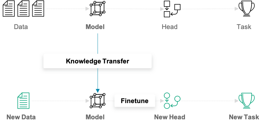
In traditional (machine) learning, we develop a model and train it on new data for every new task at hand. Transfer learning differs from this approach in that knowledge is transferred from one task to another. It is a useful approach when one is faced with the problem of too little available training data. Models that are pretrained for a similar problem can be used as a starting point for training new models. The pretrained models are referred to as base models.
In our example, a deep learning model trained on the ImageNet dataset can be used as the starting point for building a car model classifier. The main idea behind transfer learning for deep learning models is that the first layers of a network are used to extract important high-level features, which remain similar for the kind of data treated. The final layers (also known as the head) of the original network are replaced by a custom head suitable for the problem at hand. The weights in the head are initialized randomly, and the resulting network can be trained for the specific task.
There are various ways in which the base model can be treated during training. In the first step, its weights can be fixed. If the learning progress suggests the model not being flexible enough, certain layers or the entire base model can be “unfrozen” and thus made trainable. A further important aspect to note is that the input must be of the same dimensionality as the data on which the model was trained on – if the first layers of the base model are not modified.
Next, we will briefly introduce the ResNet, a popular and powerful CNN architecture for image data. Then, we will show how we used transfer learning with ResNet to do car model classification.
What is ResNet?
Training deep neural networks can quickly become challenging due to the so-called vanishing gradient problem. But what are vanishing gradients? Neural networks are commonly trained using back-propagation. This algorithm leverages the chain rule of calculus to derive gradients at deeper layers of the network by multiplying gradients from earlier layers. Since gradients get repeatedly multiplied in deep networks, they can quickly approach infinitesimally small values during back-propagation.
ResNet is a CNN network that solves the vanishing gradient problem using so-called residual blocks (you find a good explanation of why they are called ‘residual’ here). The unmodified input is passed on to the next layer in the residual block by adding it to a layer’s output (see right figure). This modification makes sure that a better information flow from the input to the deeper layers is possible. The entire ResNet architecture is depicted in the right network in the left figure below. It is plotted alongside a plain CNN and the VGG-19 network, another standard CNN architecture.
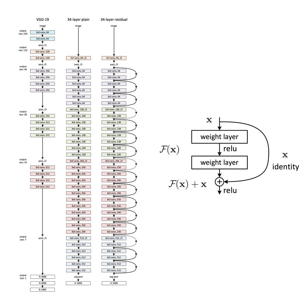
ResNet has proved to be a powerful network architecture for image classification problems. For example, an ensemble of ResNets with 152 layers won the ILSVRC 2015 image classification contest. Pretrained ResNet models of different sizes are available in the tensorflow.keras.application module, namely ResNet50, ResNet101, ResNet152 and their corresponding second versions (ResNet50V2, …). The number following the model name denotes the number of layers the networks have. The available weights are pretrained on the ImageNet dataset. The models were trained on large computing clusters using hardware accelerators for significant time periods. Transfer learning thus enables us to leverage these training results using the obtained weights as a starting point.
Classifying Car Models
As an illustrative example of how transfer learning can be applied, we treat the problem of classifying the car model given an image of the car. We will start by describing the dataset set we used and how we can filter out unwanted examples in the dataset. Next, we will go over how a data pipeline can be setup using tensorflow.data. In the second section, we will talk you through the model implementation and point out what aspects to be particularly careful about during training and prediction.
Data Preparation
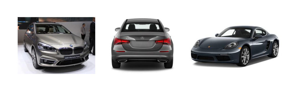
We used the dataset described in this github repo, where you can also download the entire dataset. The author built a datascraper to scrape all car images from the car connection website. He explains that many images are from the interior of the cars. As they are not wanted in the dataset, they are filtered out based on pixel color. The dataset contains 64’467 jpg images, where the file names contain information on the car’s make, model, build year, etc. For a more detailed insight on the dataset, we recommend you consult the original github repo. Three sample images are shown below.
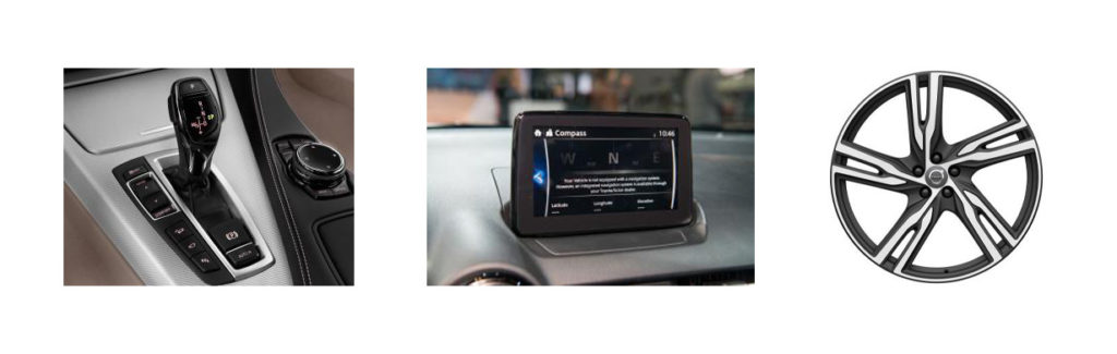
While checking through the data, we observed that the dataset still contained many unwanted images, e.g., pictures of wing mirrors, door handles, GPS panels, or lights. Examples of unwanted images can be seen below.
Thus, it is beneficial to additionally prefilter the data to clean out more of the unwanted images.
Filtering Unwanted Images Out of the Dataset
There are multiple possible approaches to filter non-car images out of the dataset:
- Use a pretrained model
- Train another model to classify car/no-car
- Train a generative network on a car dataset and use the discriminator part of the network
We decided to pursue the first approach since it is the most direct one and outstanding pretrained models are easily available. If you want to follow the second or third approach, you could, e.g., use this dataset to train the model. The referred dataset only contains images of cars but is significantly smaller than the dataset we used.
We chose the ResNet50V2 in the tensorflow.keras.applications module with the pretrained “imagenet” weights. In a first step, we must figure out the indices and classnames of the imagenet labels corresponding to car images.
# Class labels in imagenet corresponding to cars
CAR_IDX = [656, 627, 817, 511, 468, 751, 705, 757, 717, 734, 654, 675, 864, 609, 436]

CAR_CLASSES = ['minivan', 'limousine', 'sports_car', 'convertible', 'cab', 'racer', 'passenger_car', 'recreational_vehicle', 'pickup', 'police_van', 'minibus', 'moving_van', 'tow_truck', 'jeep', 'landrover', 'beach_wagon']
Next, the pretrained ResNet50V2 model is loaded.
from tensorflow.keras.applications import ResNet50V2

model = ResNet50V2(weights='imagenet')
We can then use this model to make predictions for images. The images fed to the prediction method must be scaled identically to the images used for training. The different ResNet models are trained on different input scales. It is thus essential to apply the correct image preprocessing. The module keras.application.resnet_v2 contains the method preprocess_input, which should be used when using a ResNetV2 network. This method expects the image arrays to be of type float and have values in [0, 255]. Using the appropriately preprocessed input, we can then use the built-in predict method to obtain predictions given an image stored at filename:
from tensorflow.keras.applications.resnet_v2 import preprocess_input

image = tf.io.read_file(filename)
image = tf.image.decode_jpeg(image)
image = tf.cast(image, tf.float32)
image = tf.image.resize_with_crop_or_pad(image, target_height=224, target_width=224)
image = preprocess_input(image)
predictions = model.predict(image)
There are various ideas of how the obtained predictions can be used for car detection.
- Is one of the
CAR_CLASSESamong the top k predictions? - Is the accumulated probability of the
CAR_CLASSESin the predictions greater than some defined threshold? - Specific treatment of unwanted images (e.g., detect and filter out wheels)
We show the code for comparing the accumulated probability mass over the CAR_CLASSES.
def is_car_acc_prob(predictions, thresh=THRESH, car_idx=CAR_IDX):
    """
    Determine if car on image by accumulating probabilities of car prediction and comparing to threshold

    Args:
        predictions: (?, 1000) matrix of probability predictions resulting from ResNet with imagenet weights
        thresh: threshold accumulative probability over which an image is considered a car
        car_idx: indices corresponding to cars

    Returns:
        np.array of booleans describing if car or not
    """
    predictions = np.array(predictions, dtype=float)
    car_probs = predictions[:, car_idx]
    car_probs_acc = car_probs.sum(axis=1)
    return car_probs_acc > thresh
The higher the threshold is set, the stricter the filtering procedure is. A value for the threshold that provides good results is THRESH = 0.1. This ensures we do not lose too many true car images. The choice of an appropriate threshold remains subjective, so do as you feel.
The Colab notebook that uses the function is_car_acc_prob to filter the dataset is available in the github repository.
While tuning the prefiltering procedure, we observed the following:
- Many of the car images with light backgrounds were classified as “beach wagons”. We thus decided to also consider the “beach wagon” class in imagenet as one of the
CAR_CLASSES. - Images showing the front of a car are often assigned a high probability of “grille”, which is the grating at the front of a car used for cooling. This assignment is correct but leads the procedure shown above to not consider certain car images as cars since we did not include “grille” in the
CAR_CLASSES. This problem results in the trade-off of either leaving many close-up images of car grilles in the dataset or filtering out several car images. We opted for the second approach since it yields a cleaner car dataset.
After prefiltering the images using the suggested procedure, 53’738 of 64’467 initially remain in the dataset.
Overview of the Final Datasets
The prefiltered dataset contains images from 323 car models. We decided to reduce our attention to the top 300 most frequent classes in the dataset. That makes sense since some of the least frequent classes have less than ten representatives and can thus not be reasonably split into a train, validation, and test set. Reducing the dataset to images in the top 300 classes leaves us with a dataset containing 53’536 labeled images. The class occurrences are distributed as follows:

The number of images per class (car model) ranges from 24 to slightly below 500. We can see that the dataset is very imbalanced. It is essential to keep this in mind when training and evaluating the model.
Building Data Pipelines with tf.data
Even after prefiltering and reducing to the top 300 classes, we still have numerous images left. This poses a potential problem since we can not simply load all images into the memory of our GPU at once. To tackle this problem, we will use tf.data.
tf.data and especially the tf.data.Dataset API allows creating elegant and, at the same time, very efficient input pipelines. The API contains many general methods which can be applied to load and transform potentially large datasets. tf.data.Dataset is especifically useful when training models on GPU(s). It allows for data loading from the HDD, applies transformation on-the-fly, and creates batches that are than sent to the GPU. And this is all done in a way such as the GPU never has to wait for new data.
The following functions create a tf.data.Dataset instance for our particular problem:
def construct_ds(input_files: list,
                 batch_size: int,
                 classes: list,
                 label_type: str,
                 input_size: tuple = (212, 320),
                 prefetch_size: int = 10,
                 shuffle_size: int = 32,
                 shuffle: bool = True,
                 augment: bool = False):
    """
    Function to construct a tf.data.Dataset set from list of files

    Args:
        input_files: list of files
        batch_size: number of observations in batch
        classes: list with all class labels
        input_size: size of images (output size)
        prefetch_size: buffer size (number of batches to prefetch)
        shuffle_size: shuffle size (size of buffer to shuffle from)
        shuffle: boolean specifying whether to shuffle dataset
        augment: boolean if image augmentation should be applied
        label_type: 'make' or 'model'

    Returns:
        buffered and prefetched tf.data.Dataset object with (image, label) tuple
    """
    # Create tf.data.Dataset from list of files
    ds = tf.data.Dataset.from_tensor_slices(input_files)

    # Shuffle files
    if shuffle:
        ds = ds.shuffle(buffer_size=shuffle_size)

    # Load image/labels
    ds = ds.map(lambda x: parse_file(x, classes=classes, input_size=input_size,                                                                                                                                        label_type=label_type))

    # Image augmentation
    if augment and tf.random.uniform((), minval=0, maxval=1, dtype=tf.dtypes.float32, seed=None, name=None) < 0.7:
        ds = ds.map(image_augment)

    # Batch and prefetch data
    ds = ds.batch(batch_size=batch_size)
    ds = ds.prefetch(buffer_size=prefetch_size)

    return ds
We will now describe the methods in the tf.data we used:
from_tensor_slices()is one of the available methods for the creation of a dataset. The created dataset contains slices of the given tensor, in this case, the filenames.- Next, the
shuffle()method considersbuffer_sizeelements one at a time and shuffles these items in isolation from the rest of the dataset. If shuffling of the complete dataset is required,buffer_sizemust be larger than the bumber of entries in the dataset. Shuffling is only performed ifshuffle=True. map()allows to apply arbitrary functions to the dataset. We created a functionparse_file()that can be found in the github repo. It is responsible for reading and resizing the images, inferring the labels from the file name and encoding the labels using a one-hot encoder. If the augment flag is set, the data augmentation procedure is activated. Augmentation is only applied in 70% of the cases since it is beneficial to also train the model on non-modified images. The augmentation techniques used inimage_augmentare flipping, brightness, and contrast adjustments.- Finally, the
batch()method is used to group the dataset into batches ofbatch_sizeelements and theprefetch()method enables preparing later elements while the current element is being processed and thus improves performance. If used after a call tobatch(),prefetch_sizebatches are prefetched.
Model Fine Tuning
Having defined our input pipeline, we now turn towards the model training part. Below you can see the code that can be used to instantiate a model based on the pretrained ResNet, which is available in tf.keras.applications:
from tensorflow.keras.applications import ResNet50V2
from tensorflow.keras import Model
from tensorflow.keras.layers import Dense, GlobalAveragePooling2D


class TransferModel:

    def __init__(self, shape: tuple, classes: list):
        """
        Class for transfer learning from ResNet

        Args:
            shape: Input shape as tuple (height, width, channels)
            classes: List of class labels
        """
        self.shape = shape
        self.classes = classes
        self.history = None
        self.model = None

        # Use pre-trained ResNet model
        self.base_model = ResNet50V2(include_top=False,
                                     input_shape=self.shape,
                                     weights='imagenet')

        # Allow parameter updates for all layers
        self.base_model.trainable = True

        # Add a new pooling layer on the original output
        add_to_base = self.base_model.output
        add_to_base = GlobalAveragePooling2D(data_format='channels_last', name='head_gap')(add_to_base)

        # Add new output layer as head
        new_output = Dense(len(self.classes), activation='softmax', name='head_pred')(add_to_base)

        # Define model
        self.model = Model(self.base_model.input, new_output)
A few more details on the code above:
- We first create an instance of class
tf.keras.applications.ResNet50V2. Withinclude_top=Falsewe tell the pretrained model to leave out the original head of the model (in this case designed for the classification of 1000 classes on ImageNet). base_model.trainable = Truemakes all layers trainable.- Using
tf.kerasfunctional API, we then stack a new pooling layer on top of the last convolution block of the original ResNet model. This is a necessary intermediate step before feeding the output to the final classification layer. - The final classification layer is then defined using
tf.keras.layers.Dense. We define the number of neurons to be equal to the number of desired classes. And the softmax activation function makes sure that the output is a pseudo probability in the range of(0,1].
The full version of TransferModel (see github) also contains the option to replace the base model with a VGG16 network, another standard CNN for image classification. In addition, it also allows to unfreeze only specific layers, meaning we can make the corresponding parameters trainable while leaving the others fixed. As a default, we have made all parameters trainable here.
After we defined the model, we need to configure it for training. This can be done using tf.keras.Model‘s compile()-method:
def compile(self, **kwargs):
      """
    Compile method
    """
    self.model.compile(**kwargs)
We then pass the following keyword arguments to our method:
loss = "categorical_crossentropy"for multi-class classification,optimizer = Adam(0.0001)for using the Adam optimizer fromtf.keras.optimizerswith a relatively small learning rate (more on the learning rate below), andmetrics = ["categorical_accuracy"]for training and validation monitoring.
Next, we will look at the training procedure. Therefore we define a train-method for our TransferModel-class introduced above:
from tensorflow.keras.callbacks import EarlyStopping

def train(self,
          ds_train: tf.data.Dataset,
          epochs: int,
          ds_valid: tf.data.Dataset = None,
          class_weights: np.array = None):
    """
    Trains model in ds_train with for epochs rounds

    Args:
        ds_train: training data as tf.data.Dataset
        epochs: number of epochs to train
        ds_valid: optional validation data as tf.data.Dataset
        class_weights: optional class weights to treat unbalanced classes

    Returns
        Training history from self.history
    """

    # Define early stopping as callback
    early_stopping = EarlyStopping(monitor='val_loss',
                                   min_delta=0,
                                   patience=12,
                                   restore_best_weights=True)

    callbacks = [early_stopping]

    # Fitting
    self.history = self.model.fit(ds_train,
                                  epochs=epochs,
                                  validation_data=ds_valid,
                                  callbacks=callbacks,
                                  class_weight=class_weights)

    return self.history
As our model is an instance of tensorflow.keras.Model, we can train it using the fit method. To prevent overfitting, early stopping is used by passing it to the fit method as a callback function. The patience parameter can be tuned to specify how soon early stopping should apply. The parameter stands for the number of epochs after which, if no decrease of the validation loss is registered, the training will be interrupted. Further, class weights can be passed to the fit method. Class weights allow treating unbalanced data by assigning the different classes different weights, thus allowing to increase the impact of classes with fewer training examples.
We can describe the training process using a pretrained model as follows: As the weights in the head are initialized randomly, and the weights of the base model are pretrained, the training composes of training the head from scratch and fine-tuning the pretrained model’s weights. It is recommended to use a small learning rate (e.g. 1e-4) since choosing the learning rate too large can destroy the near-optimal pretrained weights of the base model.
The training procedure can be sped up by first training for a few epochs without the base model being trainable. The purpose of these initial epochs is to adapt the heads’ weights to the problem. This speeds up the training since when training only the head, much fewer parameters are trainable and thus updated for every batch. The resulting model weights can then be used as the starting point to train the entire model, with the base model being trainable. For the car classification problem that we are considering here, applying this two-stage training did not achieve notable performance enhancement.
Model Performance Evaluation/Prediction
When using the tf.data.Dataset API, one must pay attention to the nature of the methods used. The following method in our TransferModel class can be used as a prediction method.
def predict(self, ds_new: tf.data.Dataset, proba: bool = True):
    """
    Predict class probs or labels on ds_new
    Labels are obtained by taking the most likely class given the predicted probs

    Args:
        ds_new: New data as tf.data.Dataset
        proba: Boolean if probabilities should be returned

    Returns:
        class labels or probabilities
    """

    p = self.model.predict(ds_new)

    if proba:
        return p
    else:
        return [np.argmax(x) for x in p]
It is essential that the dataset ds_new is not shuffled, or else the predictions obtained will be misaligned with the images obtained when iterating over the dataset a second time. This is the case since the flag reshuffle_each_iteration is true by default in the shuffle method’s implementation. A further effect of shuffling is that multiple calls to the take method will not return the same data. This is important when you want to check out predictions, e.g., for only one batch. A simple example where this can be seen is:
# Use construct_ds method from above to create a shuffled dataset
ds = construct_ds(..., shuffle=True)

# Take 1 batch (e.g. 32 images) of dataset: This returns a new dataset
ds_batch = ds.take(1)

# Predict labels for one batch
predictions = model.predict(ds_batch)

# Predict labels again: The result will not be the same as predictions above due to shuffling
predictions_2 = model.predict(ds_batch)
A function to plot images annotated with the corresponding predictions could look as follows:
def show_batch_with_pred(model, ds, classes, rescale=True, size=(10, 10), title=None):
      for image, label in ds.take(1):
        image_array = image.numpy()
        label_array = label.numpy()
        batch_size = image_array.shape[0]
        pred = model.predict(image, proba=False)
        for idx in range(batch_size):
            label = classes[np.argmax(label_array[idx])]
            ax = plt.subplot(np.ceil(batch_size / 4), 4, idx + 1)
            if rescale:
                plt.imshow(image_array[idx] / 255)
            else:
                plt.imshow(image_array[idx])
            plt.title("label: " + label + "\n"
                      + "prediction: " + classes[pred[idx]], fontsize=10)
            plt.axis('off')
The show_batch_with_pred method works for shuffled datasets as well, since image and label correspond to the same call to the take method.
Evaluating model perfomance can be done using keras.Model's evaluate method.
How Accurate Is Our Final Model?
The model achieves slightly above 70% categorical accuracy for the task of predicting the car model for images from 300 model classes. To better understand the model’s predictions, it is helpful to observe the confusion matrix. Below, you can see the heatmap of the model’s predictions on the validation dataset.
We restricted the heatmap to clip the confusion matrix’s entries to [0, 5], as allowing a further span did not significantly highlight any off-diagonal region. As can be seen from the heat map, one class is assigned to examples of almost all classes. That can be seen from the dark red vertical line two-thirds to the right in the figure above. Other than the class mentioned before, there are no evident biases in the predictions. We want to stress here that the categorical accuracy is generally not sufficient for a satisfactory assessment of the model’s performance, particularly in the case of imbalanced classes.
Conclusion and Next Steps
In this blog post, we have applied transfer learning using the ResNet50V2 to classify the car model from images of cars. Our model achieves 70% categorical accuracy over 300 classes.
We found unfreezing the entire base model and using a small learning rate to achieve the best results. Now, having developed a cool car classification model is great, but how can we use our model in a productive setting? Of course, we could build our custom model API using Flask or FastAPI…
But might there even be an easier, standardized way? In the second article of our series, “Deploying TensorFlow Models in Docker using TensorFlow Serving“, we discuss how this model can be deployed using TensorFlow Serving.