Create more value from your projects with the cloud.
Data science and data-driven decision-making have become a crucial part of many companies’ daily business and will become even more important in the upcoming years. Many organizations will have a cloud strategy in place by the end of 2022:
“70% of organizations will have a formal cloud strategy by 2022, and the ones that fail to adopt it will struggle”
– Gartner Research
By becoming a standard building block in all kinds of organizations, cloud technologies are getting more easily available, lowering the entry barrier for developing cloud-native applications.
In this blog entry, we will have a look at why the cloud is a good idea for data science projects. I will provide a high-level overview of the steps needed to be taken to onboard a data science project to the cloud and share some best practices from my experience to avoid common pitfalls.
I will not discuss solution patterns specific to a single cloud provider, compare them or go into detail about machine learning operations and DevOps best practices.
Data Science projects benefit from using public cloud services
One common approach to data science projects is to start by coding on local machines, crunching data, training, and snapshot-based model evaluation. This helps keeping pace at an early stage when not yet confident machine learning can solve the topic identified by the business. After having created the first version satisfying the business needs, the question arises of how to deploy that model to generate value.
Running a machine learning model in production usually can be achieved by either of two options: 1) run the model on some on-premises infrastructure. 2) run the model in a cloud environment with a cloud provider of your choice. Deploying the model on-premises might sound appealing at first and there are cases where it is a viable option. However, the cost of building and maintaining a data science specific piece of infrastructure can be quite high. This results from diverse requirements ranging from specific hardware, over managing peak loads in training phases up to additional interdependent software components.
Different cloud set-ups offer varying degrees of freedom
When using the cloud, you can choose the most suitable service level between Infrastructure as a Service (IaaS), Container as a Service (CaaS), Platform as a Service (PaaS) and Software as a Service (SaaS), usually trading off flexibility for ease of maintenance. The following picture visualizes the responsibilities in each of the service levels.
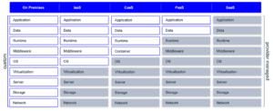
- «On-Premises» you must take care of everything yourself: ordering and setting up the necessary hardware, setting up your data pipeline and developing, running, and monitoring your applications.
- In «IaaS» the provider takes care of the hardware components and delivers a virtual machine with a fixed version of an operating system (OS).
- With «CaaS» the provider offers a container platform and orchestration solution. You can use container images from a public registry, customize them or build your own container.
- With «PaaS» services what is usually left to do is bring your data and start developing your application. Depending on whether the solution is serverless you might not even have to provide information on the sizing.
- «SaaS» solutions as the highest service level are tailored to a specific purpose and include very little effort for setup and maintenance, but offer quite limited flexibility for new features have usually to be requested from the provider
Public cloud services are already tailored to the needs of data science projects
The benefits of public cloud services include scalability, decoupling of resources and pay-as-you-go models. Those benefits are already a plus for data science applications, e.g., for scaling resources for a training run. On top of that, all 3 major cloud providers have a part of their service catalog designed specifically for data science applications, each of them with its own strengths and weaknesses.
Not only does this include special hardware like GPUs, but also integrated solutions for ML operations like automated deployments, model registries and monitoring of model performance and data drift. Many new features are constantly developed and made available. To keep up with those innovations and functionalities on-premises you would have to spend a substantial number of resources without generating direct business impact.
If you are interested in an in-depth discussion of the importance of the cloud for the success of AI projects, be sure to take a look at the white paper published on our content hub.
Onboarding your project to the cloud takes only 5 simple steps
If you are looking to get started with using the cloud for data science projects, there are a few key decisions and steps you will have to make in advance. We will take a closer look at each of those.
1. Choosing the cloud service level
BWhen choosing the service level, the most common patterns for data science applications are CaaS or PaaS. The reason is that infrastructure as a service can create high costs resulting from maintaining virtual machines or building up scalability across VMs. SaaS services on the other hand are already tailored to a specific business problem and are used instead of building your own model and application.
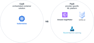
CaaS comes with the main advantage of containers, namely that containers can be deployed to any container platform of any provider. Also, when the application does not only consist of the machine learning model but needs additional micro-services or front-end components, they can all be hosted with CaaS. The downside is that similar to an on-premises roll-out, Container images for MLops tools like model registry, pipelines and model performance monitoring are not available out of the box and need to be built and integrated with the application. The larger the number of used tools and libraries, the higher the likelihood that at some point future versions will have incompatibilities or even not match at all.
PaaS services like Azure Machine Learning, Google Vertex AI or Amazon SageMaker on the other hand have all those functionalities built in. The downside of these services is that they all come with complex cost structures and are specific to the respective cloud provider. Depending on the project requirements the PaaS services may in some special cases feel too restrictive.
When comparing CaaS and PaaS it mostly comes down to the tradeoff between flexibility and a higher level of vendor lock-in. Higher vendor lock-in comes with paying an extra premium for the sake of included features, increased compatibility and rise in the speed of development. Higher flexibility on the other hand comes at the cost of increased integration and maintenance effort.
2. Making your data available in cloud
Usually, the first step to making your data available is to upload a snapshot of the data to a cloud object storage. These are well integrated with other services and can later be replaced by a more suitable data storage solution with little effort. Once the results from the machine learning model are suitable from a business perspective, data engineers should set up a process to automatically keep your data up to date.
3. Building a pipeline for preprocessing
In any data science project, one crucial step is building a robust pipeline for data preprocessing. This ensures your data is clean and ready for modeling, which will save you time and effort in the long run. A best practice is to set up a continuous integration and continuous delivery (CICD) pipeline to automate deployment and testing of your preprocessing and to make it part of your DevOps cycle. The cloud helps you automatically scale your pipelines to deal with any amount of data needed for the training of your model.
4. Training and evaluating trained models
In this stage, the preprocessing pipeline is extended by adding modeling components. This includes hyper-parameter tuning which cloud services once again support by scaling resources and storing the results of each training experiment for easier comparison. All cloud providers offer an automated machine learning service. This can be used either to generate the first version of a model quickly and compare performance on the data across multiple model types. This way you can quickly assess if the data and preprocessing suffice to tackle the business problem. Besides that, the result can be utilized as a benchmark for the data scientist. The best model should be stored in a model registry for deployment and transparency.
In case a model has already been trained locally or on-premises, it is possible to skip the training and just load the model into the model registry.
5. Serving models to business users
The final and likely most important step is serving the model to your business unit to create value from it. All cloud providers offer solutions to deploy the model in a scalable manner with little effort. Finally, all pieces created in the earlier steps from automatically provisioning the most recent data over applying preprocessing and feeding the data into the deployed model come together.
Now we have gone through the steps of how to onboard your data science project. With these 5 steps you are well on the way with moving your data science workflow to the cloud. To avoid some of the common pitfalls, here are some learnings from my personal experiences I would like to share, which can positively impact your project’s success.
Make your move to the cloud even easier with these useful tips
Start using the cloud early in the process.
By starting early, the team can familiarize themselves with the platform’s features. This will help you make the most of its capabilities and avoid potential problems and heavy refactoring down the road
Make sure your data is accessible.
This may seem like a no-brainer, but it is important to make sure your data is easily accessible when you move to the cloud. This is especially true in a setup where your data is generated on-premises and needs to be transferred to the cloud.
Consider using serverless computing.
Serverless computing is a great option for data science projects because it allows you to scale your resources up or down as needed without having to provision or manage any servers.
Don’t forget about security.
While all cloud providers offer some of the most up-to-date IT-security setups, some of them are easy to miss during configuration and can expose your project to needless risk.
Monitor your cloud expenses.
Coming from on-premises, optimization is often about peak resource usage because hardware or licenses are limited. With scalability and pay-as-you-go, this paradigm shifts stronger towards optimizing costs. Optimizing costs is usually not the first activity to do when starting a project but keeping an eye on the costs can prevent unpleasant surprises and be used at a later stage to make a cloud application even more cost-effective.
Take your data science projects to new heights with the cloud
If you’re starting your next data science project, doing so into the cloud is a great option. It is scalable, flexible, and offers a variety of services that can help you get the most out of your project. Cloud based architectures are a modern way of developing applications, that are expected to grow even more important in the future.
Following the steps presented will help you on that journey and support you in keeping up with the newest trends and developments. Plus, with the tips provided, you can avoid many of the common pitfalls that may occur on the way. So, if you’re looking for a way to get the most out of your data science project, the cloud is definitely worth considering.
Why bother? AI and the climate crisis
According to the newest report from the Intergovernmental Panel on Climate Change (IPCC) in August 2021, “it is unequivocal that human influence has warmed the atmosphere, ocean and land” [1]. Climate change also occurs faster than previously thought. Regarding most recent estimations, the average global surface temperature increased by 1.07°C from 2010 to 2019 compared to 1850 to 1900 due to human influence. Furthermore, the atmospheric CO2 concentrations in 2019 “were higher than at any time in at least 2 million years” [1].
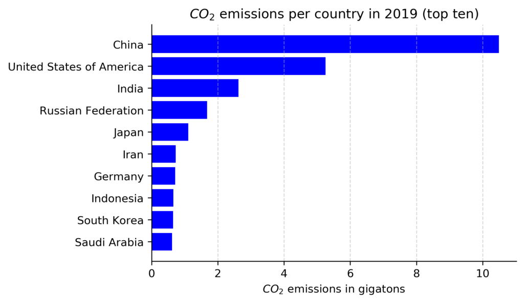
Still, global carbon emissions are rising, although there was a slight decrease in 2020 [2], probably due to the coronavirus and its economic effects. In 2019, 36.7 gigatons (Gt) CO2 were emitted worldwide [2]. Be aware that one Gt is one billion tons. To achieve the 1.5 °C goal with an estimated probability of about 80%, we have only 300 Gts left at the beginning of 2020 [1]. As both 2020 and 2021 are over and assuming carbon emissions of about 35 Gts for each year, the remaining budget is about 230 Gt CO2. If the yearly amount stayed constant over the next years, the remaining carbon budget would be exhausted in about seven years.
In 2019, China, the USA, and India were the most emitting countries. Overall, Germany is responsible for only about 2% of all global emissions, but it was still in seventh place with about 0.7 Gt in 2019 (see graph below). Altogether, the top ten most emitting countries account for about two-thirds of all carbon emissions in 2019 [2]. Most of these countries are highly industrialized and will likely enhance their usage of artificial intelligence (AI) to strengthen their economies during the following decades.
Using AI to reduce carbon emissions
So, what about AI and carbon emissions? Well, the usage of AI is two sides of the same coin [3]. On the one hand, AI has a great potential to reduce carbon emissions by providing more accurate predictions or improving processes in many different fields. For example, AI can be applied to predict intemperate weather events, optimize supply chains, or monitor peatlands [4, 5].
According to a recent estimation of Microsoft and PwC, the usage of AI for environmental applications can save up to 4.4% of all greenhouse gas emissions worldwide by 2030 [6].
In absolute numbers, the usage of AI for environmental applications can reduce worldwide greenhouse gas emissions by 0.9 – 2.4 Gts of CO2e. This amount is equivalent to the estimated annual emissions of Australia, Canada, and Japan together in 2030 [7]. To be clear, greenhouse gases also include other emitted gases like methane that also reinforce the earth’s greenhouse effect. To easily measure all of them, they are often declared as equivalents to CO2 and hence abbreviated as CO2e.
AI’s carbon footprint
Despite the great potential of AI to reduce carbon emissions, the usage of AI itself also emits CO2, which is the other side of the coin. From 2012 to 2018, the estimated amount of computation used to train deep learning models has increased by 300.000 (see graph below, [8]). Hence, research, training, and deployment of AI models require an increasing amount of energy and hardware, of course. Both produce carbon emissions and thus contribute to climate change.
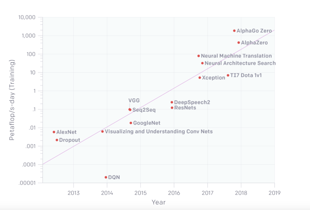
Note: Graph taken from [8].
Unfortunately, I could not find a study that estimates the overall carbon emissions of AI. Still, there are some estimations of the CO2 or CO2e emissions of some Natural Language Processing (NLP) models that have become increasingly accurate and hence popular during recent years [9]. According to the following table, the final training of Google’s BERT model roughly emitted as much CO2e as one passenger on their flight from New York to San Francisco. Of course, the training of other NLP models – like Transformerbig – emitted far less, but the final training of a model is only the last part of finding the best model. Prior to the final training, many different models are tried to find the best parameters. Accordingly, this neural architecture search for the Transformerbig model emitted about five times the CO2e emissions as an average car in its lifetime. Now, you may look at the estimated CO2e emissions of GPT-3 and imagine how much emissions resulted from the related neural architecture search.
| Human emissions | AI emissions | ||
|---|---|---|---|
| Example | CO2e emissions (tons) | NLP model training | CO2e emissions (tons) |
| One passenger air traveling New York San Francisco |
0.90 | Transformerbig | 0.09 |
| Average human life one year |
5.00 | BERTbase | 0.65 |
| Average American life one year |
16.40 | GPT-3 | 84.74 |
| Average car lifetime incl. fuel |
57.15 | Neural architecture search for Transformerbig |
284.02 |
Note: All values extracted from [9], except the value of for GPT-3 [17]
What you, as a data scientist, can do the reduce your carbon footprint
Overall, there are many ways you, as a data scientist, can reduce your carbon footprint during the training and deployment of AI models. As the most important areas of AI are currently machine learning (ML) and deep learning (DL), different ways to measure and reduce the carbon footprint of these models are described in the following.
1. Be aware of the negative consequences and report them
It may sound simple but being aware of the negative consequences of searching, training, and deploying ML and DL models is the first step to reducing your carbon emissions. It is essential to understand how AI negatively impacts our environment to take the extra effort and be willing to report carbon emissions systematically, which is needed to tackle climate change [8, 9, 10]. So, if you skipped the first part about AI and the climate crisis, go back and read it. It’s worth it!
2. Measure the carbon footprint of your code
To make carbon emissions of your ML and DL models explicit, they need to be measured. Currently, there is no standardized framework to measure all sustainability aspects of AI, but one is currently formed [11]. Until there is a holistic framework, you can start by making energy consumption and related carbon emissions explicit [12]. Probably, some of the most elaborated packages to compute ML and DL models are implemented in the programming language Python. Although Python is not the most efficient programming language [13], it was again rated the most popular programming language in the PYPL index in September 2021 [14]. Accordingly, there are even three Python packages that you can use to track the carbon emissions of training your models:
- CodeCarbon [15, 16]
- CarbonTracker [17]
- Experiment Impact Tracker [18]
Based on my perception, CodeCarbon and CarbonTracker seem to be the easiest ones to use. Furthermore, CodeCarbon can easily be combined with TensorFlow and CarbonTracker with PyTorch. Therefore, you find an example for each package below.
I trained a simple multilayer perceptron with two hidden layers and 256 neurons using the MNIST data set for both packages. To simulate a CPU- and GPU-based computation, I trained the model with TensorFlow and CodeCarbon on my local machine (15-inches MacBook Pro from 2018 and 6 Intel Core i7 CPUs) and the one with PyTorch and Carbontracker in a Google Colab using a Tesla K80 GPU. First, you find the TensorFlow and CodeCarbon code below.
# import needed packages
import tensorflow as tf
from codecarbon import EmissionsTracker

# prepare model training
mnist = tf.keras.datasets.mnist

(x_train, y_train), (x_test, y_test) = mnist.load_data()
x_train, x_test = x_train / 255.0, x_test / 255.0


model = tf.keras.models.Sequential(
    [
        tf.keras.layers.Flatten(input_shape=(28, 28)),
        tf.keras.layers.Dense(256, activation="relu"),
        tf.keras.layers.Dense(256, activation="relu"),
        tf.keras.layers.Dense(10, activation="softmax"),
    ]
)

loss_fn = tf.keras.losses.SparseCategoricalCrossentropy(from_logits=True)

model.compile(optimizer="adam", loss=loss_fn, metrics=["accuracy"])

# train model and track carbon emissions
tracker = EmissionsTracker()
tracker.start()
model.fit(x_train, y_train, epochs=10)
emissions: float = tracker.stop()
print(emissions)
After executing the code above, Codecarbon creates a csv file as output which includes different output parameters like computation duration in seconds, total power consumed by the underlying infrastructure in kWh and the related CO2e emissions in kg. The training of my model took 112.15 seconds, consumed 0.00068 kWh, and created 0.00047 kg of CO2e.
Regarding PyTorch and CarbonTracker, I used this Google Colab notebook as the basic setup. To incorporate the tracking of carbon emissions and make the two models comparable, I changed a few details of the notebook. First, I changed the model in step 2 (Define Network) from a convolutional neural network to the multilayer perceptron (I kept the class name CNN to make the rest of the notebook still work):
 class CNN(nn.Module):
  """A simple MLP model."""

  @nn.compact
  def __call__(self, x):
    x = x.reshape((x.shape[0], -1))  # flatten
    x = nn.Dense(features=256)(x)
    x = nn.relu(x)
    x = nn.Dense(features=256)(x)
    x = nn.relu(x)
    x = nn.Dense(features=10)(x)
    x = nn.log_softmax(x)
    return x
Second, I inserted the installation and import of CarbonTracker as well as the tracking of the carbon emissions in step 14 (Train and evaluate):
 !pip install carbontracker

from carbontracker.tracker import CarbonTracker

tracker = CarbonTracker(epochs=num_epochs)
for epoch in range(1, num_epochs + 1):
tracker.epoch_start()
# Use a separate PRNG key to permute image data during shuffling
rng, input_rng = jax.random.split(rng)
# Run an optimization step over a training batch
state = train_epoch(state, train_ds, batch_size, epoch, input_rng)
# Evaluate on the test set after each training epoch
test_loss, test_accuracy = eval_model(state.params, test_ds)
print(' test epoch: %d, loss: %.2f, accuracy: %.2f' % (
epoch, test_loss, test_accuracy * 100))
tracker.epoch_end()
tracker.stop()After executing the whole notebook, CarbonTracker prints the following output after the first training epoch is finished.
 train epoch: 1, loss: 0.2999, accuracy: 91.25
 test epoch: 1, loss: 0.22, accuracy: 93.42
CarbonTracker:
Actual consumption for 1 epoch(s):
       Time:  0:00:15
       Energy: 0.000397 kWh
       CO2eq: 0.116738 g
       This is equivalent to:
       0.000970 km travelled by car
CarbonTracker:
Predicted consumption for 10 epoch(s):
       Time:  0:02:30
       Energy: 0.003968 kWh
       CO2eq: 1.167384 g
       This is equivalent to:
       0.009696 km travelled by car
As expected, the GPU needed more energy and produced more carbon emissions. The energy consumption was 6 times higher and the carbon emissions about 2.5 times higher compared to my local CPUs. Obviously, the increased energy consumption is related to the increased computation time that was 2.5 minutes for the GPU but only less than 2 minutes for the CPUs. Overall, both packages provide all needed information to assess and report carbon emissions and related information.
3. Compare different regions of cloud providers
In recent years, the training and deployment of ML or DL models in the cloud have become more important compared to local computations. Clearly, one of the reasons is the increased need for computation power [8]. Accessing GPUs in the cloud is, for most companies, faster and cheaper than building their own data center. Of course, data centers of cloud providers also need hardware and energy for computation. It is estimated that about 1% of worldwide electricity demand is produced by data centers [19]. The usage of every hardware, regardless of its location, produces carbon emissions, and that’s why it is also important to measure carbon emissions emitted by training and deployment of ML and DL models in the cloud.
Currently, there are two different CO2e calculators that can easily be used to calculate carbon emissions in the cloud [20, 21]. The good news is that all three big cloud providers – AWS, Azure, and GCP – are incorporated in both calculators. To find out which of the three big cloud providers and which European region is best, I used the first calculator – ML CO2 Impact [20] – to calculate the CO2e emissions for the final training of GPT-3. The final model training of GPT-3 required 310 GPUs (NVIDIA Tesla V100 PCIe) running non-stop for 90 days [17]. To compute the estimated emissions of the different providers and regions, I chose the available option “Tesla V100-PCIE-16GB” as GPU. The results of the calculations can be found in the following table.
| Google Cloud Computing | AWS Cloud Computing | Microsoft Azure | |||
|---|---|---|---|---|---|
| Region | CO2e emissions (tons) | Region | CO2e emissions (tons) | Region | CO2e emissions (tons) |
| europe-west1 | 54.2 | EU – Frankfurt | 122.5 | France Central | 20.1 |
| europe-west2 | 124.5 | EU – Ireland | 124.5 | France South | 20.1 |
| europe-west3 | 122.5 | EU – London | 124.5 | North Europe | 124.5 |
| europe-west4 | 114.5 | EU – Paris | 20.1 | West Europe | 114.5 |
| europe-west6 | 4.0 | EU – Stockholm | 10.0 | UK West | 124.5 |
| europe-north1 | 42.2 | UK South | 124.5 | ||
Overall, at least two findings are fascinating. First, even within the same cloud provider, the chosen region has a massive impact on the estimated CO2e emissions. The most significant difference is present for GCP with a factor of more than 30. This huge difference is partly due to the small emissions of 4 tons in the region europe-west6, which are also the smallest emissions overall. Interestingly, such a huge factor of 30 is a lot more than those described in scientific papers, which are factors of 5 to 10 [12]. Second, some estimated values are equal, which shows that some kind of simplification was used for these estimations. Therefore, you should treat the absolute values with caution, but the difference between the regions still holds as they are all based on the same (simplified) way of calculation.
Finally, to choose the cloud provider with a minimal carbon footprint in total, it is also essential to consider the sustainability strategies of the cloud providers. In this area, GCP and Azure seem to have more effective strategies for the future compared to AWS [22, 23] and have already reached 100% renewable energy with offsets and energy certificates so far. Still, none of them uses 100% renewable energy itself (see table 2 in [9]). From an environmental perspective, I personally prefer GCP because their strategy most convinced me. Furthermore, GCP has implemented a hint for “regions with the lowest carbon impact inside Cloud Console location selectors“ since 2021 [24]. These kinds of help indicate the importance of this topic to GCP.
4. Train and deploy with care
Finally, there are many other helpful hints and tricks related to the training and deployment of ML and DL models that can help you minimize your carbon footprint as a data scientist.
- Practice to be sparse! New research that combines DL models with state-of-the-art findings in neuroscience can reduce computation times by up to 100 times and save lots of carbon emissions [25].
- Search for simpler and less computing-intensive models with comparable accuracy and use them if appropriate. For example, there is a smaller and faster version of BERT available called DistilBERT with comparable accuracy values [26]
- Consider transfer learning and foundation models [10] to maximize accuracy and minimize computations at the same time.
- Consider Federated learning to reduce carbon emissions [27].
- Don’t just think of the accuracy of your model; consider efficiency as well. Always ponder if a 1% increase in accuracy is worth the additional environmental impact [9, 12].
- If the region of best hyperparameters is still unknown, use random or Bayesian hyperparameter search instead of grid search [9, 20].
- If your model will be retrained periodically after deployment, choose the training interval consciously. Regarding the associated business case, it may be enough to provide a newly trained model each month and not each week.
Conclusion
Human beings and their greenhouse gas emissions influence our climate and warm the world. AI can and should be part of the solution to tackle climate change. Still, we need to keep an eye on its carbon footprint to make sure that it will be part of the solution and not part of the problem.
As a data scientist, you can do a lot. You can inform yourself and others about the positive possibilities and negative consequences of using AI. Furthermore, you can measure and explicitly state the carbon emissions of your models. You can describe your efforts to minimize their carbon footprint, too. Finally, you can also choose your cloud provider consciously and, for example, check if there are simpler models that result in a comparable accuracy but with fewer emissions.
Recently, we at statworx have formed a new initiative called AI and Environment to incorporate these aspects in our daily work as data scientists. If you want to know more about it, just get in touch with us!
References
- https://www.ipcc.ch/report/ar6/wg1/downloads/report/IPCC_AR6_WGI_SPM_final.pdf
- http://www.globalcarbonatlas.org/en/CO2-emissions
- https://doi.org/10.1007/s43681-021-00043-6
- https://arxiv.org/pdf/1906.05433.pdf
- https://www.pwc.co.uk/sustainability-climate-change/assets/pdf/how-ai-can-enable-a-sustainable-future.pdf
- Harness Artificial Intelligence
- https://climateactiontracker.org/
- https://arxiv.org/pdf/1907.10597.pdf
- https://arxiv.org/pdf/1906.02243.pdf
- https://arxiv.org/pdf/2108.07258.pdf
- https://algorithmwatch.org/de/sustain/
- https://arxiv.org/ftp/arxiv/papers/2104/2104.10350.pdf
- https://stefanos1316.github.io/my_curriculum_vitae/GKS17.pdf
- https://pypl.github.io/PYPL.html
- https://codecarbon.io/
- https://mlco2.github.io/codecarbon/index.html
- https://arxiv.org/pdf/2007.03051.pdf
- https://github.com/Breakend/experiment-impact-tracker
- https://www.iea.org/reports/data-centres-and-data-transmission-networks
- https://mlco2.github.io/impact/#co2eq
- http://www.green-algorithms.org/
- https://blog.container-solutions.com/the-green-cloud-how-climate-friendly-is-your-cloud-provider
- https://www.wired.com/story/amazon-google-microsoft-green-clouds-and-hyperscale-data-centers/
- https://cloud.google.com/blog/topics/sustainability/pick-the-google-cloud-region-with-the-lowest-co2)
- https://arxiv.org/abs/2112.13896
- https://arxiv.org/abs/1910.01108
- https://flower.dev/blog/2021-07-01-what-is-the-carbon-footprint-of-federated-learning
Management Summary
Deploying and monitoring machine learning projects is a complex undertaking. In addition to the consistent documentation of model parameters and the associated evaluation metrics, the main challenge is to transfer the desired model into a productive environment. If several people are involved in the development, additional synchronization problems arise concerning the models’ development environments and version statuses. For this reason, tools for the efficient management of model results through to extensive training and inference pipelines are required. In this article, we present the typical challenges along the machine learning workflow and describe a possible solution platform with MLflow. In addition, we present three different scenarios that can be used to professionalize machine learning workflows:
- Entry-level Variant: Model parameters and performance metrics are logged via a R/Python API and clearly presented in a GUI. In addition, the trained models are stored as artifacts and can be made available via APIs.
- Advanced Model Management: In addition to tracking parameters and metrics, certain models are logged and versioned. This enables consistent monitoring and simplifies the deployment of selected model versions.
- Collaborative Workflow Management: Encapsulating Machine Learning projects as packages or Git repositories and the accompanying local reproducibility of development environments enable smooth development of Machine Learning projects with multiple stakeholders.
Depending on the maturity of your machine learning project, these three scenarios can serve as inspiration for a potential machine learning workflow. We have elaborated each scenario in detail for better understanding and provide recommendations regarding the APIs and deployment environments to use.
Challenges Along the Machine Learning Workflow
Training machine learning models is becoming easier and easier. Meanwhile, a variety of open-source tools enable efficient data preparation as well as increasingly simple model training and deployment.
The added value for companies comes primarily from the systematic interaction of model training, in the form of model identification, hyperparameter tuning and fitting on the training data, and deployment, i.e., making the model available for inference tasks. This interaction is often not established as a continuous process, especially in the early phases of machine learning initiative development. However, a model can only generate added value in the long term if a stable production process is implemented from model training, through its validation, to testing and deployment. If this process is implemented correctly, complex dependencies and costly maintenance work in the long term can arise during the operational start-up of the model [2]. The following risks are particularly noteworthy in this regard.
1. Ensuring Synchronicity
Often, in an exploratory context, data preparation and modeling workflows are developed locally. Different configurations of development environments or even the use of different technologies make it difficult to reproduce results, especially between developers or teams. In addition, there are potential dangers concerning the compatibility of the workflow if several scripts must be executed in a logical sequence. Without an appropriate version control logic, the synchronization effort afterward can only be guaranteed with great effort.
2. Documentation Effort
To evaluate the performance of the model, model metrics are often calculated following training. These depend on various factors, such as the parameterization of the model or the influencing factors used. This meta-information about the model is often not stored centrally. However, for systematic further development and improvement of a model, it is mandatory to have an overview of the parameterization and performance of all past training runs.
3. Heterogeneity of Model Formats
In addition to managing model parameters and results, there is the challenge of subsequently transferring the model to the production environment. If different models from multiple packages are used for training, deployment can quickly become cumbersome and error-prone due to different packages and versions.
4. Recovery of Prior Results
In a typical machine learning project, the situation often arises that a model is developed over a long period of time. For example, new features may be used, or entirely new architectures may be evaluated. These experiments do not necessarily lead to better results. If experiments are not versioned cleanly, there is a risk that old results can no longer be reproduced.
Various tools have been developed in recent years to solve these and other challenges in the handling and management of machine learning workflows, such as TensorFlow TFX, cortex, Marvin, or MLFlow. The latter, in particular, is currently one of the most widely used solutions.
MLflow is an open-source project with the goal to combine the best of existing ML platforms to make the integration to existing ML libraries, algorithms, and deployment tools as straightforward as possible [3]. In the following, we will introduce the main MLflow modules and discuss how machine learning workflows can be mapped via MLflow.
MLflow Services
MLflow consists of four components: MLflow Tracking, MLflow Models, MLflow Projects, and MLflow Registry. Depending on the requirements of the experimental and deployment scenario, all services can be used together, or individual components can be isolated.
With MLflow Tracking, all hyperparameters, metrics (model performance), and artifacts, such as charts, can be logged. MLflow Tracking provides the ability to collect presets, parameters, and results for collective monitoring for each training or scoring run of a model. The logged results can be visualized in a GUI or alternatively accessed via a REST API.
The MLflow Models module acts as an interface between technologies and enables simplified deployment. Depending on its type, a model is stored as a binary, e.g., a pure Python function, or as a Keras or H2O model. One speaks here of the so-called model flavors. Furthermore, MLflow Models provides support for model deployment on various machine learning cloud services, e.g., for AzureML and Amazon Sagemaker.
MLflow Projects are used to encapsulate individual ML projects in a package or Git repository. The basic configurations of the respective environment are defined via a YAML file. This can be used, for example, to control how exactly the conda environment is parameterized, which is created when MLflow is executed. MLflow Projects allows experiments that have been developed locally to be executed on other computers in the same environment. This is an advantage, for example, when developing in smaller teams.
MLflow Registry provides a centralized model management. Selected MLflow models can be registered and versioned in it. A staging workflow enables a controlled transfer of models into the productive environment. The entire process can be controlled via a GUI or a REST API.
Examples of Machine Learning Pipelines Using MLflow
In the following, three different ML workflow scenarios are presented using the above MLflow modules. These increase in complexity from scenario to scenario. In all scenarios, a dataset is loaded into a development environment using a Python script, processed, and a machine learning model is trained. The last step in all scenarios is a deployment of the ML model in an exemplary production environment.
1. Scenario – Entry-Level Variant
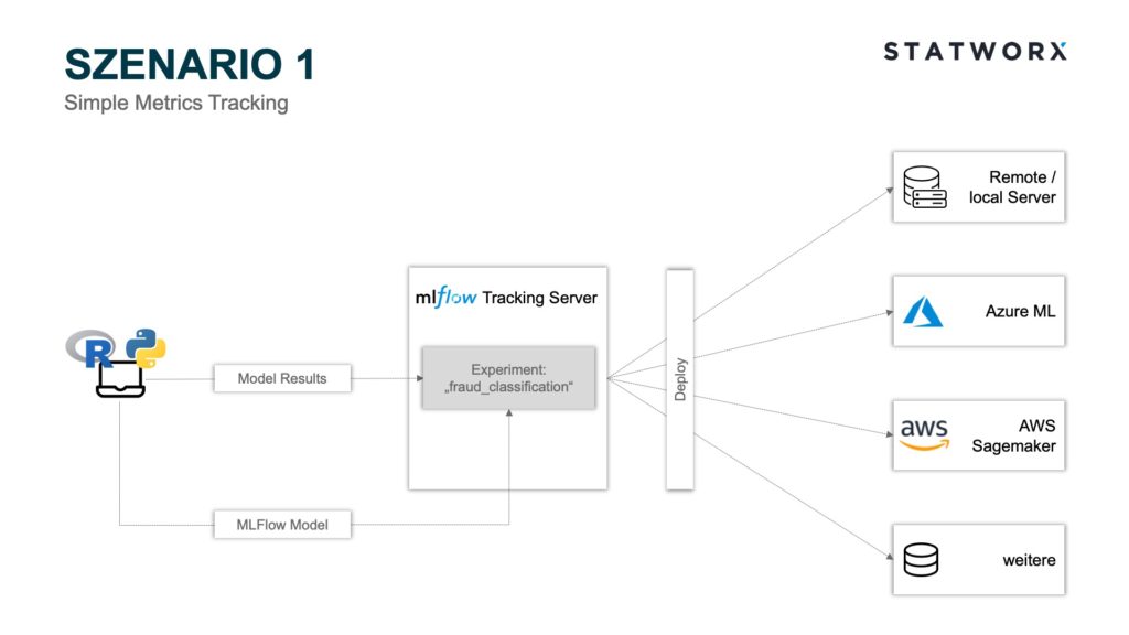 Scenario 1 – Simple Metrics Tracking
Scenario 1 uses the MLflow Tracking and MLflow Models modules. Using the Python API, the model parameters and metrics of the individual runs can be stored on the MLflow Tracking Server Backend Store, and the corresponding MLflow Model File can be stored as an artifact on the MLflow Tracking Server Artifact Store. Each run is assigned to an experiment. For example, an experiment could be called ‘fraud_classification’, and a run would be a specific ML model with a certain hyperparameter configuration and the corresponding metrics. Each run is stored with a unique RunID.
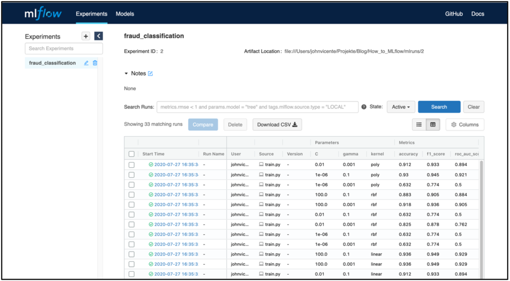
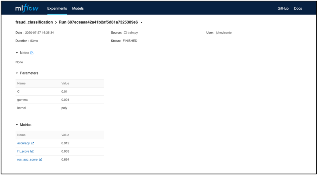
In the screenshot above, the MLflow Tracking UI is shown as an example after executing a model training. The server is hosted locally in this example. Of course, it is also possible to host the server remotely. For example in a Docker container within a virtual machine. In addition to the parameters and model metrics, the time of the model training, as well as the user and the name of the underlying script, are also logged. Clicking on a specific run also displays additional information, such as the RunID and the model training duration.
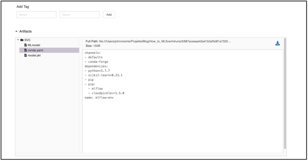
If you have logged other artifacts in addition to the metrics, such as the model, the MLflow Model Artifact is also displayed in the Run view. In the example, a model from the sklearn.svm package was used. The MLmodel file contains metadata with information about how the model should be loaded. In addition to this, a conda.yaml is created that contains all the package dependencies of the environment at training time. The model itself is located as a serialized version under model.pkl and contains the model parameters optimized on the training data.
The deployment of the trained model can now be done in several ways. For example, suppose one wants to deploy the model with the best accuracy metric. In that case, the MLflow tracking server can be accessed via the Python API mlflow.list_run_infos to identify the RunID of the desired model. Now, the path to the desired artifact can be assembled, and the model loaded via, for example, the Python package pickle. This workflow can now be triggered via a Dockerfile, allowing flexible deployment to the infrastructure of your choice. MLflow offers additional separate APIs for deployment on Microsoft Azure and AWS. For example, if the model is to be deployed on AzureML, an Azure ML container image can be created using the Python API mlflow.azureml.build_image, which can be deployed as a web service to Azure Container Instances or Azure Kubernetes Service. In addition to the MLflow Tracking Server, it is also possible to use other storage systems for the artifact, such as Amazon S3, Azure Blob Storage, Google Cloud Storage, SFTP Server, NFS, and HDFS.
2. Scenario – Advanced Model Management
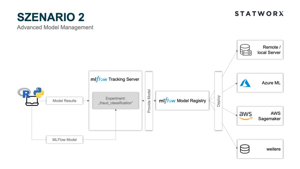 Scenario 2 – Advanced Model Management
Scenario 2 includes, in addition to the modules used in scenario 1, MLflow Model Registry as a model management component. Here, it is possible to register and process the models logged there from specific runs. These steps can be controlled via the API or GUI. A basic requirement to use the Model Registry is deploying the MLflow Tracking Server Backend Store as Database Backend Store. To register a model via the GUI, select a specific run and scroll to the artifact overview.
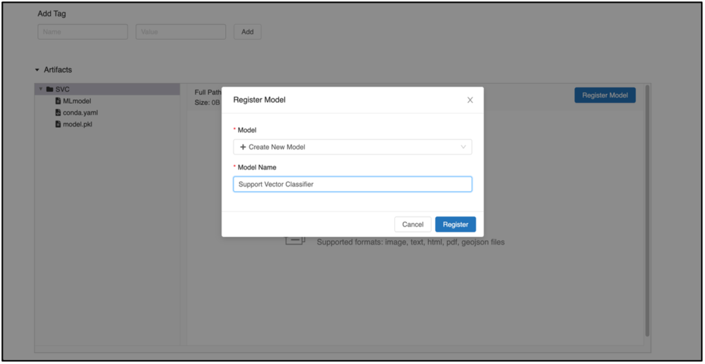
Clicking on Register Model opens a new window in which a model can be registered. If you want to register a new version of an already existing model, select the desired model from the dropdown field. Otherwise, a new model can be created at any time. After clicking the Register button, the previously registered model appears in the Models tab with corresponding versioning.
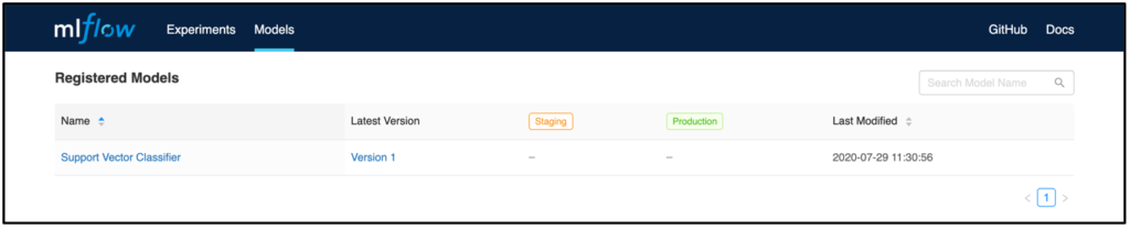
Each model includes an overview page that shows all past versions. This is useful, for example, to track which models were in production when.
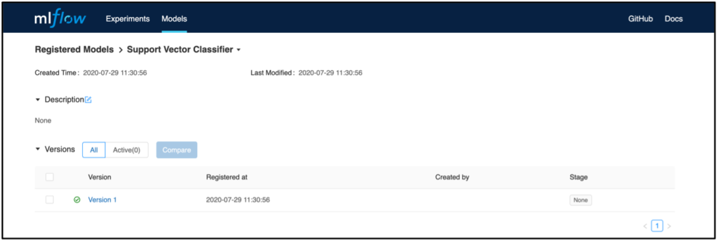
If you now select a model version, you will get to an overview where, for example, a model description can be added. The Source Run link also takes you to the run from which the model was registered. Here you will also find the associated artifact, which can be used later for deployment.
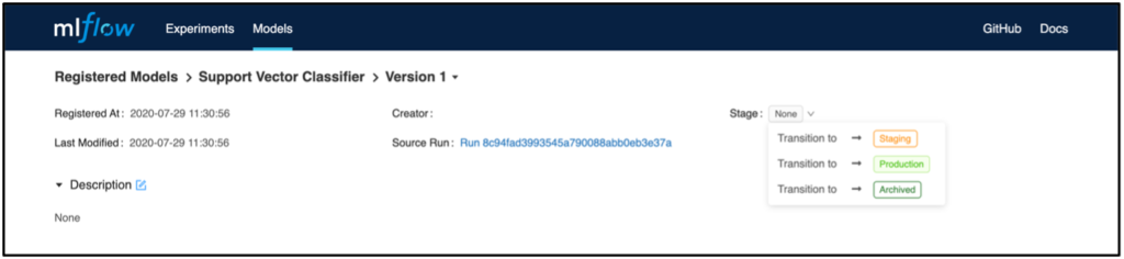
In addition, individual model versions can be categorized into defined phases in the Stage area. This feature can be used, for example, to determine which model is currently being used in production or is to be transferred there. For deployment, in contrast to scenario 1, versioning and staging status can be used to identify and deploy the appropriate model. For this, the Python API MlflowClient().search_model_versions can be used, for example, to filter the desired model and its associated RunID. Similar to scenario 1, deployment can then be completed to, for example, AWS Sagemaker or AzureML via the respective Python APIs.
3. Scenario – Collaborative Workflow Management
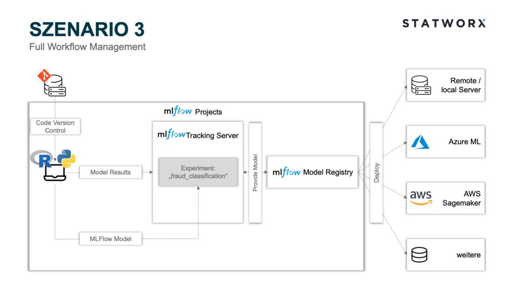 Scenario 3 – Full Workflow Management
In addition to the modules used in scenario 2, scenario 3 also includes the MLflow Projects module. As already explained, MLflow Projects are particularly well suited for collaborative work. Any Git repository or local environment can act as a project and be controlled by an MLproject file. Here, package dependencies can be recorded in a conda.yaml, and the MLproject file can be accessed when starting the project. Then the corresponding conda environment is created with all dependencies before training and logging the model. This avoids the need for manual alignment of the development environments of all developers involved and also guarantees standardized and comparable results of all runs. Especially the latter is necessary for the deployment context since it cannot be guaranteed that different package versions produce the same model artifacts. Instead of a conda environment, a Docker environment can also be defined using a Dockerfile. This offers the advantage that package dependencies independent of Python can also be defined. Likewise, MLflow Projects allow the use of different commit hashes or branch names to use other project states, provided a Git repository is used.
An interesting use case is the modularized development of machine learning training pipelines [4]. For example, data preparation can be decoupled from model training and developed in parallel, while another team uses a different branch name to train the model. In this case, only a different branch name must be used as a parameter when starting the project in the MLflow Projects file. The final data preparation can then be pushed to the same branch name used for model training and would thus already be fully implemented in the training pipeline. The deployment can also be controlled as a sub-module within the project pipeline through a Python script via the ML Project File and can be carried out analogous to scenario 1 or 2 on a platform of your choice.
Conclusion and Outlook
MLflow offers a flexible way to make the machine learning workflow robust against the typical challenges in the daily life of a data scientist, such as synchronization problems due to different development environments or missing model management. Depending on the maturity level of the existing machine learning workflow, various services from the MLflow portfolio can be used to achieve a higher level of professionalization.
In the article, three machine learning workflows, ascending in complexity, were presented as examples. From simple logging of results in an interactive UI to more complex, modular modeling pipelines, MLflow services can support it. Logically, there are also synergies outside the MLflow ecosystem with other tools, such as Docker/Kubernetes for model scaling or even Jenkins for CI/CD pipeline control. If there is further interest in MLOps challenges and best practices, I refer you to the webinar on MLOps by our CEO Sebastian Heinz, which we provide free of charge.
Resources
- https://www.aitrends.com/machine-learning/mlops-not-just-ml-business-new-competitive-frontier/
- Hidden Technical Debt in Machine Learning Systems (2014) von D. Sculley et al., (https://papers.nips.cc/paper/5656-hidden-technical-debt-in-machine-learning-systems.pdf)
- https://databricks.com/blog/2018/06/05/introducing-mlflow-an-open-source-machine-learning-platform.html
- https://mlflow.org/docs/latest/projects.html#building-multistep-workflows
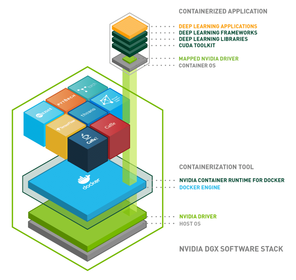
In a recent project at STATWORX, I’ve developed a large scale deep learning application for image classification using Keras and Tensorflow. After developing the model, we needed to deploy it in a quite complex pipeline of data acquisition and preparation routines in a cloud environment. We decided to deploy the model on a prediction server that exposes the model through an API. Thereby, we came across NVIDIA TensorRT Server (TRT Server), a serious alternative to good old TF Serving (which is an awesome product, by the way!). After checking the pros and cons, we decided to give TRT Server a shot. TRT Server has sevaral advantages over TF Serving, such as optimized inference speed, easy model management and ressource allocation, versioning and parallel inference handling. Furthermore, TensorRT Server is not “limited” to TensorFlow (and Keras) models. It can serve models from all major deep learning frameworks, such as TensorFlow, MxNet, pytorch, theano, Caffe and CNTK.
Despite the load of cool features, I found it a bit cumbersome to set up the TRT server. The installation and documentation is scattered to quite a few repositories, documetation guides and blog posts. That is why I decided to write this blog post about setting up the server and get your predictions going!
NVIDIA TensorRT Server
TensorRT Inference Server is NVIDIA’s cutting edge server product to put deep learning models into production. It is part of the NVIDIA’s TensorRT inferencing platform and provides a scaleable, production-ready solution for serving your deep learning models from all major frameworks. It is based on NVIDIA Docker and contains everything that is required to run the server from the inside of the container. Furthermore, NVIDIA Docker allows for using GPUs inside a Docker container, which, in most cases, significantly speeds up model inference. Talking about speed – TRT Server can be considerably faster than TF Serving and allows for multiple inferences from multiple models at the same time, using CUDA streams to exploit GPU scheduling and serialization (see image below).
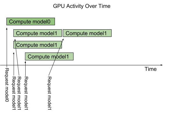
With TRT Server you can specify the number of concurrent inference computations using so called instance groups that can be configured on the model level (see section “Model Configuration File”) . For example, if you are serving two models and one model gets significantly more inference requests, you can assign more GPU ressources to this model allowing you to compute more multiple requests in parallel. Furthermore, instance groups allow you to specify, whether a model should be executed on CPU or GPU, which can be a very interesting feature in more complex serving environments. Overall, TRT Server has a bunch of great features that makes it interesting for production usage.
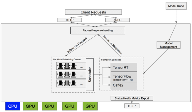
The upper image illustrates the general architecture of the server. One can see the HTTP and gRPC interfaces that allow you to integrate your models into other applications that are connected to the server over LAN or WAN. Pretty cool! Furthermore, the server exposes a couple of sanity features such as health status checks etc., that also come in handy in production.
Setting up the Server
As mentioned before, TensorRT Server lives inside a NVIDIA Docker container. In order to get things going, you need to complete several installation steps (in case you are starting with a blank machine, like here). The overall process is quite long and requires a certain amount of “general cloud, network and IT knowledge”. I hope, that the following steps make the installation and setup process clear to you.
Launch a Deep Learning VM on Google Cloud
For my project, I used a Google Deep Learning VM that comes with preinstalled CUDA as well as TensorFlow libraries. You can launch a cloud VM using the Google Cloud SDK or in the GCP console (which is pretty easy to use, in my opinion). The installation of the GCP SDK can be found here. Please note, that it might take some time until you can connect to the server because of the CUDA installation process, which takes several minutes. You can check the status of the VM in the cloud logging console.
# Create project
gcloud projects create tensorrt-server

# Start instance with deep learning image
gcloud compute instances create tensorrt-server-vm
	--project tensorrt-server
	--zone your-zone
	--machine-type n1-standard-4
	--create-disk='size=50'
	--image-project=deeplearning-platform-release
	--image-family tf-latest-gpu
	--accelerator='type=nvidia-tesla-k80,count=1'
	--metadata='install-nvidia-driver=True'
	--maintenance-policy TERMINATE
After successfully setting up your instance, you can SSH into the VM using the terminal. From there you can execute all the neccessary steps to install the required components.
# SSH into instance
gcloud compute ssh tensorrt-server-vm --project tensorrt-server --zone your-zone
Note: Of course, you have to adapt the script for your project and instance names.
Install Docker
After setting up the GCP cloud VM, you have to install the Docker service on your machine. The Google Deep Learning VM uses Debian as OS. You can use the following code to install Docker on the VM.
# Install Docker
sudo apt-get update
sudo apt-get install
    apt-transport-https
    ca-certificates
    curl
    software-properties-common
curl -fsSL https://download.docker.com/linux/ubuntu/gpg | sudo apt-key add -
sudo add-apt-repository
   "deb [arch=amd64] https://download.docker.com/linux/ubuntu
   $(lsb_release -cs)
   stable"
sudo apt-get update
sudo apt-get install docker-ce
You can verify that Docker has been successfully installed by running the following command.
sudo docker run --rm hello-world
You should see a “Hello World!” from the docker container which should give you something like this:
Unable to find image 'hello-world:latest' locally
latest: Pulling from library/hello-world
d1725b59e92d: Already exists
Digest: sha256:0add3ace90ecb4adbf7777e9aacf18357296e799f81cabc9fde470971e499788
Status: Downloaded newer image for hello-world:latest

Hello from Docker!
This message shows that your installation appears to be working correctly.

To generate this message, Docker took the following steps:
 1. The Docker client contacted the Docker daemon.
 2. The Docker daemon pulled the "hello-world" image from the Docker Hub.
    (amd64)
 3. The Docker daemon created a new container from that image which runs the
    executable that produces the output you are currently reading.
 4. The Docker daemon streamed that output to the Docker client, which sent it
    to your terminal.

To try something more ambitious, you can run an Ubuntu container with:
 $ docker run -it ubuntu bash

Share images, automate workflows, and more with a free Docker ID:
 https://hub.docker.com/

For more examples and ideas, visit:
 https://docs.docker.com/get-started/
Congratulations, you’ve just installed Docker successfully!
Install NVIDIA Docker
Unfortunately, Docker has no “out of the box” support for GPUs connected to the host system. Therefore, the installation of the NVIDIA Docker runtime is required to use TensorRT Server’s GPU capabilities within a containerized environment. NVIDIA Docker is also used for TF Serving, if you want to use your GPUs for model inference. The following figure illustrates the architecture of the NVIDIA Docker Runtime.
You can see, that the NVIDIA Docker Runtime is layered around the Docker engine allowing you to use standard Docker as well as NVIDIA Docker containers on your system.
Since the NVIDIA Docker Runtime is a proprietary product of NVIDIA, you have to register at NVIDIA GPU Cloud (NGC) to get an API key in order to install and download it. To authenticate against NGC execute the following command in the server command line:
# Login to NGC
sudo docker login nvcr.io
You will be prompted for username and API key. For username you have to enter $oauthtoken, the password is the generated API key. After you have successfully logged in, you can install the NVIDIA Docker components. Following the instructions on the NVIDIA Docker GitHub repo, you can install NVIDIA Docker by executing the following script (Ubuntu 14.04/16.04/18.04, Debian Jessie/Stretch).
# If you have nvidia-docker 1.0 installed: we need to remove it and all existing GPU containers
docker volume ls -q -f driver=nvidia-docker | xargs -r -I{} -n1 docker ps -q -a -f volume={} | xargs -r docker rm -f
sudo apt-get purge -y nvidia-docker

# Add the package repositories
curl -s -L https://nvidia.github.io/nvidia-docker/gpgkey |
  sudo apt-key add -
distribution=$(. /etc/os-release;echo $ID$VERSION_ID)
curl -s -L https://nvidia.github.io/nvidia-docker/$distribution/nvidia-docker.list |
  sudo tee /etc/apt/sources.list.d/nvidia-docker.list
sudo apt-get update

# Install nvidia-docker2 and reload the Docker daemon configuration
sudo apt-get install -y nvidia-docker2
sudo pkill -SIGHUP dockerd

# Test nvidia-smi with the latest official CUDA image
sudo docker run --runtime=nvidia --rm nvidia/cuda:9.0-base nvidia-smi
Installing TensorRT Server
The next step, after successfully installing NVIDIA Docker, is to install TensorRT Server. It can be pulled from the NVIDIA Container Registry (NCR). Again, you need to be authenticated against NGC to perform this action.
# Pull TensorRT Server (make sure to check the current version)
sudo docker pull nvcr.io/nvidia/tensorrtserver:18.09-py3
After pulling the image, TRT Server is ready to be started on your cloud machine. The next step is to create a model that will be served by TRT Server.
Model Deployment
After installing the required technical components and pulling the TRT Server container you need to take care of your model and the deployment. TensorRT Server manages it’s models in a folder on your server, the so called model repository.
Setting up the Model Repository
The model repository contains your exported TensorFlow / Keras etc. model graphs in a specific folder structure. For each model in the model repository, a subfolder with the corresponding model name needs to be defined. Within those model subfolders, the model schema files (config.pbtxt), label definitions (labels.txt) as well as model version subfolders are located. Those subfolders allow you to manage and serve different model versions. The file labels.txt contains strings of the target labels in appropriate order, corresponding to the output layer of the model. Within the version subfolder a file named model.graphdef (the exported protobuf graph) is stored. model.graphdef is actually a frozen tensorflow graph, that is created after exporting a TensorFlow model and needs to be named accordingly.
Remark: I did not manage to get a working serving from a tensoflow.python.saved_model.simple_save() or tensorflow.python.saved_model.builder.SavedModelBuilder() export with TRT Server due to some variable initialization error. We therefore use the “freezing graph” approach, which converts all TensorFlow variable inside a graph to constants and outputs everything into a single file (which is model.graphdef).
/models
|-   model_1/
|--      config.pbtxt
|--      labels.txt
|--      1/
|---		model.graphdef
Since the model repository is just a folder, it can be located anywhere the TRT Server host has a network connection to. For exmaple, you can store your exported model graphs in a cloud repository or a local folder on your machine. New models can be exported and deployed there in order to be servable through the TRT Server.
Model Configuration File
Within your model repository, the model configuration file (config.pbtxt) sets important parameters for each model on the TRT Server. It contains technical information about your servable model and is required for the model to be loaded properly. There are sevaral things you can control here:
name: "model_1"
platform: "tensorflow_graphdef"
max_batch_size: 64
input [
   {
      name: "dense_1_input"
      data_type: TYPE_FP32
      dims: [ 5 ]
   }
]
output [
   {
      name: "dense_2_output"
      data_type: TYPE_FP32
      dims: [ 2 ]
      label_filename: "labels.txt"
   }
]
instance_group [
   {
      kind: KIND_GPU
      count: 4
   }
]
First, name defines the tag under the model is reachable on the server. This has to be the name of your model folder in the model repository. platform defines the framework, the model was built with. If you are using TensorFlow or Keras, there are two options: (1) tensorflow_savedmodel and tensorflow_graphdef. As mentioned before, I used tensorflow_graphdef (see my remark at the end of the previous section). batch_size, as the name says, controls the batch size for your predictions. input defines your model’s input layer node name, such as the name of the input layer (yes, you should name your layers and nodes in TensorFlow or Keras), the data_type, currently only supporting numeric types, such as TYPE_FP16, TYPE_FP32, TYPE_FP64 and the input dims. Correspondingly, output defines your model’s output layer name, it’s data_type and dims. You can specify a labels.txt file that holds the labels of the output neurons in appropriate order. Since we only have two output classes here, the file looks simply like this:
class_0
class_1
Each row defines a single class label. Note, that the file does not contain any header. The last section instance_group lets you define specific GPU (KIND_GPU)or CPU (KIND_CPU) ressources to your model. In the example file, there are 4 concurrent GPU threads assigned to the model, allowing for four simultaneous predictions.
Building a simple model for serving
In order to serve a model through TensorRT server, you’ll first need – well – a model. I’ve prepared a small script that builds a simple MLP for demonstration purposes in Keras. I’ve already used TRT Server successfully with bigger models such as InceptionResNetV2 or ResNet50 in production and it worked very well.
from sklearn.datasets import make_classification
from sklearn.model_selection import train_test_split
from sklearn.preprocessing import StandardScaler
from keras.models import Sequential
from keras.layers import InputLayer, Dense
from keras.callbacks import EarlyStopping, ModelCheckpoint
from keras.utils import to_categorical

# Make toy data
X, y = make_classification(n_samples=1000, n_features=5)

# Make target categorical
y = to_categorical(y)

# Train test split
X_train, X_test, y_train, y_test = train_test_split(X, y)

# Scale inputs
scaler = StandardScaler()
X_train = scaler.fit_transform(X_train)
X_test = scaler.transform(X_test)

# Model definition
model_1 = Sequential()
model_1.add(Dense(input_shape=(X_train.shape[1], ),
                  units=16, activation='relu', name='dense_1'))
model_1.add(Dense(units=2, activation='softmax', name='dense_2'))
model_1.compile(optimizer='adam', loss='categorical_crossentropy')

# Early stopping
early_stopping = EarlyStopping(patience=5)
model_checkpoint = ModelCheckpoint(filepath='model_checkpoint.h5',
                                   save_best_only=True,
                                   save_weights_only=True)
callbacks = [early_stopping, model_checkpoint]

# Fit model and load best weights
model_1.fit(x=X_train, y=y_train, validation_data=(X_test, y_test),
            epochs=50, batch_size=32, callbacks=callbacks)

# Load best weights after early stopping
model_1.load_weights('model_checkpoint.h5')

# Export model
model_1.save('model_1.h5')
The script builds some toy data using sklearn.datasets.make_classification and fits a single layer MLP to the data. After fitting, the model gets saved for further treatment in a separate export script.
Freezing the graph for serving
Serving a Keras (TensorFlow) model works by exporting the model graph as a separate protobuf file (.pb-file extension). A simple way to export the model into a single file, that contains all the weights of the network, is to “freeze” the graph and write it to disk. Thereby, all the tf.Variables in the graph are converted to tf.constant which are stored together with the graph in a single file. I’ve modified this script for that purpose.
import os
import shutil
import keras.backend as K
import tensorflow as tf
from keras.models import load_model
from tensorflow.python.framework import graph_util
from tensorflow.python.framework import graph_io

def freeze_model(model, path):
    """ Freezes the graph for serving as protobuf """
    # Remove folder if present
    if os.path.isdir(path):
        shutil.rmtree(path)
        os.mkdir(path)
        shutil.copy('config.pbtxt', path)
        shutil.copy('labels.txt', path)
    # Disable Keras learning phase
    K.set_learning_phase(0)
    # Load model
    model_export = load_model(model)
    # Get Keras sessions
    sess = K.get_session()
    # Output node name
    pred_node_names = ['dense_2_output']
    # Dummy op to rename the output node
    dummy = tf.identity(input=model_export.outputs[0], name=pred_node_names)
    # Convert all variables to constants
    graph_export = graph_util.convert_variables_to_constants(
        sess=sess,
        input_graph_def=sess.graph.as_graph_def(),
        output_node_names=pred_node_names)
    graph_io.write_graph(graph_or_graph_def=graph_export,
                         logdir=path + '/1',
                         name='model.graphdef',
                         as_text=False)

# Freeze Model
freeze_model(model='model_1.h5', path='model_1')

# Upload to GCP
os.system('gcloud compute scp model_1 tensorrt-server-vm:~/models/ --project tensorrt-server --zone us-west1-b --recurse')
The freeze_model() function takes the path to the saved Keras model file model_1.h5 as well as the path for the graph to be exported. Furthermore, I’ve enhanced the function in order to build the required model repository folder structure containing the version subfolder, config.pbtxt as well as labels.txt, both stored in my project folder. The function loads the model and exports the graph into the defined destination. In order to do so, you need to define the output node’s name and then convert all variables in the graph to constants using graph_util.convert_variables_to_constants, which uses the respective Keras backend session, that has to be fetched using K.get_session(). Furthermore, it is important to disable the Keras learning mode using K.set_learning_phase(0) prior to export. Lastly, I’ve included a small CLI command that uploads my model folder to my GCP instance to the model repository /models.
Starting the Server
Now that everything is installed, set up and configured, it is (finally) time to launch our TRT prediciton server. The following command starts the NVIDIA Docker container and maps the model repository to the container.
sudo nvidia-docker run --rm --name trtserver -p 8000:8000 -p 8001:8001
-v ~/models:/models nvcr.io/nvidia/tensorrtserver:18.09-py3 trtserver
--model-store=/models
--rm removes existing containers of the same name, given by --name. -p exposes ports 8000 (REST) and 8001 (gRPC) on the host and maps them to the respective container ports. -v mounts the model repository folder on the host, which is /models in my case, to the container into /models, which is then referenced by --model-store as the location to look for servable model graphs. If everything goes fine you should see similar console output as below. If you don’t want to see the output of the server, you can start the container in detached model using the -d flag on startup.
===============================
== TensorRT Inference Server ==
===============================

NVIDIA Release 18.09 (build 688039)

Copyright (c) 2018, NVIDIA CORPORATION.  All rights reserved.
Copyright 2018 The TensorFlow Authors.  All rights reserved.

Various files include modifications (c) NVIDIA CORPORATION.  All rights reserved.
NVIDIA modifications are covered by the license terms that apply to the underlying
project or file.

NOTE: The SHMEM allocation limit is set to the default of 64MB.  This may be
   insufficient for the inference server.  NVIDIA recommends the use of the following flags:
   nvidia-docker run --shm-size=1g --ulimit memlock=-1 --ulimit stack=67108864 ...

I1014 10:38:55.951258 1 server.cc:631] Initializing TensorRT Inference Server
I1014 10:38:55.951339 1 server.cc:680] Reporting prometheus metrics on port 8002
I1014 10:38:56.524257 1 metrics.cc:129] found 1 GPUs supported power usage metric
I1014 10:38:57.141885 1 metrics.cc:139]   GPU 0: Tesla K80
I1014 10:38:57.142555 1 server.cc:884] Starting server 'inference:0' listening on
I1014 10:38:57.142583 1 server.cc:888]  localhost:8001 for gRPC requests
I1014 10:38:57.143381 1 server.cc:898]  localhost:8000 for HTTP requests
[warn] getaddrinfo: address family for nodename not supported
[evhttp_server.cc : 235] RAW: Entering the event loop ...
I1014 10:38:57.880877 1 server_core.cc:465] Adding/updating models.
I1014 10:38:57.880908 1 server_core.cc:520]  (Re-)adding model: model_1
I1014 10:38:57.981276 1 basic_manager.cc:739] Successfully reserved resources to load servable {name: model_1 version: 1}
I1014 10:38:57.981313 1 loader_harness.cc:66] Approving load for servable version {name: model_1 version: 1}
I1014 10:38:57.981326 1 loader_harness.cc:74] Loading servable version {name: model_1 version: 1}
I1014 10:38:57.982034 1 base_bundle.cc:180] Creating instance model_1_0_0_gpu0 on GPU 0 (3.7) using model.savedmodel
I1014 10:38:57.982108 1 bundle_shim.cc:360] Attempting to load native SavedModelBundle in bundle-shim from: /models/model_1/1/model.savedmodel
I1014 10:38:57.982138 1 reader.cc:31] Reading SavedModel from: /models/model_1/1/model.savedmodel
I1014 10:38:57.983817 1 reader.cc:54] Reading meta graph with tags { serve }
I1014 10:38:58.041695 1 cuda_gpu_executor.cc:890] successful NUMA node read from SysFS had negative value (-1), but there must be at least one NUMA node, so returning NUMA node zero
I1014 10:38:58.042145 1 gpu_device.cc:1405] Found device 0 with properties:
name: Tesla K80 major: 3 minor: 7 memoryClockRate(GHz): 0.8235
pciBusID: 0000:00:04.0
totalMemory: 11.17GiB freeMemory: 11.10GiB
I1014 10:38:58.042177 1 gpu_device.cc:1455] Ignoring visible gpu device (device: 0, name: Tesla K80, pci bus id: 0000:00:04.0, compute capability: 3.7) with Cuda compute capability 3.7. The minimum required Cuda capability is 5.2.
I1014 10:38:58.042192 1 gpu_device.cc:965] Device interconnect StreamExecutor with strength 1 edge matrix:
I1014 10:38:58.042200 1 gpu_device.cc:971]      0
I1014 10:38:58.042207 1 gpu_device.cc:984] 0:   N
I1014 10:38:58.067349 1 loader.cc:113] Restoring SavedModel bundle.
I1014 10:38:58.074260 1 loader.cc:148] Running LegacyInitOp on SavedModel bundle.
I1014 10:38:58.074302 1 loader.cc:233] SavedModel load for tags { serve }; Status: success. Took 92161 microseconds.
I1014 10:38:58.075314 1 gpu_device.cc:1455] Ignoring visible gpu device (device: 0, name: Tesla K80, pci bus id: 0000:00:04.0, compute capability: 3.7) with Cuda compute capability 3.7. The minimum required Cuda capability is 5.2.
I1014 10:38:58.075343 1 gpu_device.cc:965] Device interconnect StreamExecutor with strength 1 edge matrix:
I1014 10:38:58.075348 1 gpu_device.cc:971]      0
I1014 10:38:58.075353 1 gpu_device.cc:984] 0:   N
I1014 10:38:58.083451 1 loader_harness.cc:86] Successfully loaded servable version {name: model_1 version: 1}
There is also a warning showing that you should start the container using the following arguments
--shm-size=1g --ulimit memlock=-1 --ulimit stack=67108864
You can do this of course. However, in this example I did not use them.
Installing the Python Client
Now it is time to test our prediction server. TensorRT Server comes with several client libraries that allow you to send data to the server and get predictions. The recommended method of building the client libraries is again – Docker. To use the Docker container, that contains the client libraries, you need to clone the respective GitHub repo using:
git clone https://github.com/NVIDIA/dl-inference-server.git
Then, cd into the folder dl-inference-server and run
docker build -t inference_server_clients .
This will build the container on your machine (takes some time). To use the client libraries within the container on your host, you need to mount a folder to the container. First, start the container in an interactive session (-it flag)
docker run --name tensorrtclient --rm -it -v /tmp:/tmp/host inference_server_clients
Then, run the following commands in the container’s shell (you may have to create /tmp/host first):
cp build/image_client /tmp/host/.
cp build/perf_client /tmp/host/.
cp build/dist/dist/tensorrtserver-*.whl /tmp/host/.
cd /tmp/host
The code above copies the prebuilt image_client and perf_client libraries into the mounted folder and makes it accessible from the host system. Lastly, you need to install the Python client library using
pip install tensorrtserver-0.6.0-cp35-cp35m-linux_x86_64.whl
on the container system. Finally! That’s it, we’re ready to go (sounds like it was an easy way)!
Inference using the Python Client
Using Python, you can easily perform predictions using the client library. In order to send data to the server, you need an InferContext() from the inference_server.api module that takes the TRT Server IP and port as well as the desired model name. If you are using the TRT Server in the cloud, make sure, that you have appropriate firewall rules allowing for traffic on ports 8000 and 8001.
from tensorrtserver.api import *
import numpy as np

# Some parameters
outputs = 2
batch_size = 1

# Init client
trt_host = '123.456.789.0:8000' # local or remote IP of TRT Server
model_name = 'model_1'
ctx = InferContext(trt_host, ProtocolType.HTTP, model_name)

# Sample some random data
data = np.float32(np.random.normal(0, 1, [1, 5]))

# Get prediction
# Layer names correspond to the names in config.pbtxt
response = ctx.run(
    {'dense_1_input': data},
    {'dense_2_output': (InferContext.ResultFormat.CLASS, outputs)},
    batch_size)

# Result
print(response)
{'output0': [[(0, 1.0, 'class_0'), (1, 0.0, 'class_1')]]}
Note: It is important that the data you are sending to the server matches the floating point precision, previously defined for the input layer in the model definition file. Furthermore, the names of the input and output layers must exactly match those of your model. If everything went well, ctx.run() returns a dictionary of predicted values, which you would further postprocess according to your needs.
Conclusion and Outlook
Wow, that was quite a ride! However, TensorRT Server is a great product for putting your deep learning models into production. It is fast, scaleable and full of neat features for production usage. I did not go into details regarding inference performance. If you’re interested in more, make sure to check out this blog post from NVIDIA. I must admit, that in comparison to TRT Server, TF Serving is much more handy when it comes to installation, model deployment and usage. However, compared to TRT Server it lacks some functionalities that are handy in production. Bottom line: my team and I will definitely add TRT Server to our production tool stack for deep learning models.
If you have any comments or questions on my story, feel free to comment below! I will try to answer them. Also, feel free to use my code or share this story with your peers on social platforms of your choice.
If you’re interested in more content like this, join our mailing list, constantly bringing you new data science, machine learning and AI reads and treats from me and my team at STATWORX right into your inbox!
Lastly, follow me on LinkedIn or Twitter, if you’re interested to connect with me.
References
- pictures are taken from this NVIDIA Developer blog
Google AutoML Vision is a state-of-the-art cloud service from Google that is able to build deep learning models for image recognition completely fully automated and from scratch. In this post, Google AutoML Vision is used to build an image classification model on the Zalando Fashion-MNIST dataset, a recent variant of the classical MNIST dataset, which is considered to be more difficult to learn for ML models, compared to digit MNIST.
During the benchmark, both AutoML Vision training modes, “free” (0 $, limited to 1 hour computing time) and “paid” (approx. 500 $, 24 hours computing time) were used and evaluated:
Thereby, the free AutoML model achieved a macro AUC of 96.4% and an accuracy score of 88.9% on the test set at a computing time of approx. 30 minutes (early stopping). The paid AutoML model achieved a macro AUC of 98.5% on the test set with an accuracy score of 93.9%.
Introduction
Recently, there is a growing interest in automated machine learning solutions. Products like H2O Driverless AI or DataRobot, just to name a few, aim at corporate customers and continue to make their way into professional data science teams and environments. For many use cases, AutoML solutions can significantly speed up time-2-model cycles and therefore allow for faster iteration and deployment of models (and actually start saving / making money in production).
Automated machine learning solutions will transform the data science and ML landscape substantially in the next 3-5 years. Thereby, many ML models or applications that nowadays require respective human input or expertise will likely be partly or fully automated by AI / ML models themselves. Likely, this will also yield a decline in overall demand for “classical” data science profiles in favor of more engineering and operations related data science roles that bring models into production.
A recent example of the rapid advancements in automated machine learning this is the development of deep learning image recognition models. Not too long ago, building an image classifier was a very challenging task that only few people were acutally capable of doing. Due to computational, methodological and software advances, barriers have been dramatically lowered to the point where you can build your first deep learning model with Keras in 10 lines of Python code and getting “okayish” results.
Undoubtly, there will still be many ML applications and cases that cannot be (fully) automated in the near future. Those cases will likely be more complex because basic ML tasks, such as fitting a classifier to a simple dataset, can and will easily be automated by machines.
At this point, first attempts in moving into the direction of machine learning automation are made. Google as well as other companies are investing in AutoML research and product development. One of the first professional automated ML products on the market is Google AutoML Vision.
Google AutoML Vision
Google AutoML Vision (at this point in beta) is Google’s cloud service for automated machine learning for image classification tasks. Using AutoML Vision, you can train and evaluate deep learning models without any knowledge of coding, neural networks or whatsoever.
AutoML Vision operates in the Google Cloud and can be used either based on a graphical user interface or via, REST, command line or Python. AutoML Vision implements strategies from Neural Architecture Search (NAS), currently a scientific field of high interest in deep learning research. NAS is based on the idea that another model, typically a neural network or reinforcement learning model, is designing the architecture of the neural network that aims to solve the machine learning task. Cornerstones in NAS research were the paper from Zoph et at. (2017) as well as Pham et al. (2018). The latter has also been implemented in the Python package autokeras (currently in pre-release phase) and makes neural architecture search feasible on desktop computers with a single GPU opposed to 500 GPUs used in Zoph et al.
The idea that an algorithm is able to discover architectures of a neural network seems very promising, however is still kind of limited due to computational contraints (I hope you don’t mind that I consider a 500-1000 GPU cluster as as computational contraint). But how good does neural architecture search actually work in a pre-market-ready product?
Benchmark
In the following section, Google AutoML vision is used to build an image recognition model based on the Fashion-MNIST dataset.
Dataset
The Fashion-MNIST dataset is supposed to serve as a “drop-in replacement” for the traditional MNIST dataset and has been open-sourced by Europe’s online fashion giant Zalando‘s research department (check the Fashion-MNIST GitHub repo and the Zalando reseach website). It contains 60,000 training and 10,000 test images of 10 different clothing categories (tops, pants, shoes etc.). Just like in MNIST, each image is a 28×28 grayscale image. It shares the same image size and structure of training and test images. Below are some examples from the dataset:

The makers of Fashion-MNIST argue, that nowadays the traditional MNIST dataset is a too simple task to solve – even simple convolutional neural networks achieve >99% accuracy on the test set whereas classical ML algorithms easily score >97%. For this and other reasons, Fashion-MNIST was created.
The Fashion-MNIST repo contains helper functions for loading the data as well as some scripts for benchmarking and testing your models. Also, there’s a neat visualization of an ebmedding of the data on the repo. After cloning, you can import the Fashion-MNIST data using a simple Python function (check the code in the next section) and start to build your model.
Using Google AutoML Vision
Preparing the data
AutoML offers two ways of data ingestion: (1) upload a zip file that contains the training images in different folders, corresponding to the respective labels or (2) upload a CSV file that contains the Goolge cloud storage (GS) filepaths, labels and optionally the data partition for training, validation and test set. I decided to go with the CSV file because you can define the data partition (flag names are TRAIN, VALIDATION and TEST) in order to keep control over the experiment. Below is the required structure of the CSV file that needs to be uploaded to AutoML Vision (without the header!).
| partition | file | label |
|---|---|---|
| TRAIN | gs://bucket-name/folder/image_0.jpg | 0 |
| TRAIN | gs://bucket-name/folder/image_1.jpg | 2 |
| … | … | |
| VALIDATION | gs://bucket-name/folder/image_22201.jpg | 7 |
| VALIDATION | gs://bucket-name/folder/image_22202.jpg | 9 |
| … | … | … |
| TEST | gs://bucket-name/folder/image_69998.jpg | 4 |
| TEST | gs://bucket-name/folder/image_69999.jpg | 1 |
Just like MNIST, Fashion-MNIST data contains the pixel values of the respective images. To actually upload image files, I developed a short python script that takes care of the image creation, export and upload to GCP. The script iterates over each row of the Fashion-MNIST dataset, exports the image and uploads it into a Google Cloud storage bucket.
import os
import gzip
import numpy as np
import pandas as pd
from google.cloud import storage
from keras.preprocessing.image import array_to_img


def load_mnist(path, kind='train'):
    """Load MNIST data from `path`"""
    labels_path = os.path.join(path,
                               '%s-labels-idx1-ubyte.gz'
                               % kind)
    images_path = os.path.join(path,
                               '%s-images-idx3-ubyte.gz'
                               % kind)

    with gzip.open(labels_path, 'rb') as lbpath:
        labels = np.frombuffer(lbpath.read(), dtype=np.uint8,
                               offset=8)

    with gzip.open(images_path, 'rb') as imgpath:
        images = np.frombuffer(imgpath.read(), dtype=np.uint8,
                               offset=16).reshape(len(labels), 784)

    return images, labels


# Import training data
X_train, y_train = load_mnist(path='data', kind='train')
X_test, y_test = load_mnist(path='data', kind='t10k')

# Split validation data
from sklearn.model_selection import train_test_split
X_train, X_valid, y_train, y_valid = train_test_split(X_train, y_train, test_size=10000)

# Dataset placeholder
files = pd.DataFrame({'part': np.concatenate([np.repeat('TRAIN', 50000),
                                              np.repeat('VALIDATION', 10000),
                                              np.repeat('TEST', 10000)]),
                      'file': np.repeat('file', 70000),
                      'label': np.repeat('label', 70000)})

# Stack training and test data into single arrays
X_data = np.vstack([X_train, X_valid, X_test])
y_data = np.concatenate([y_train, y_valid, y_test])

# GS path
gs_path = 'gs://secret/fashionmnist'

# Storgae client
storage_client = storage.Client.from_service_account_json(json_credentials_path='secret.json')
bucket = storage_client.get_bucket('secret-bucket')

# Fill matrix
for i, x in enumerate(X_data):
    # Console print
    if i % 1000 == 0:
        print('Uploading image {image}'.format(image=i))
    # Reshape and export image
    img = array_to_img(x=x.reshape(28, 28, 1))
    img.save(fp='fashionmnist' + '/' + 'image_' + str(i) + '.jpg')
    # Add info to data frame
    files.iloc[i, 1] = gs_path + '/' + 'image_' + str(i) + '.jpg'
    files.iloc[i, 2] = y_data[i]
    # Upload to GCP
    blob = bucket.blob('fashionmnist/' + 'image_' + str(i) + '.jpg')
    blob.upload_from_filename('fashionmnist/' + 'image_' + str(i) + '.jpg')
    # Delete image file
    os.remove('fashionmnist/' + 'image_' + str(i) + '.jpg')

# Export CSV file
files.to_csv(path_or_buf='fashionmnist.csv', header=False, index=False)
The function load_mnist is from the Fashion-MNIST repository and imports the training and test arrays into Python. After importing the training set, 10,000 examples are sampled and sotored as validation data using train_test_split from sklean.model_selection. The training, validation and test arrays are then stacked into X_data in order to have a single object for iteration. A placeholder DataFrame is initialized to store the required information (partition, filepath and label), required by AutoML Vision. storage from google.cloud connects to GCP using a service account json file (which I will, of course, not share here). Finally, the main process takes place, iterating over X_data, generating an image for each row, saving it to disk, uploading it to GCP and deleting the image since it is no longer needed. Lastly, I uploaded the exported CSV file into the Google Cloud storage bucket of the project.
Getting into AutoML
AutoML Vision is currently in Beta, which means that you have to apply before trying it out. Since me and my colleagues are currently exploring the usage of automated machine learning in a computer vision project for one of our customers, I already have access to AutoML Vision through the GCP console.
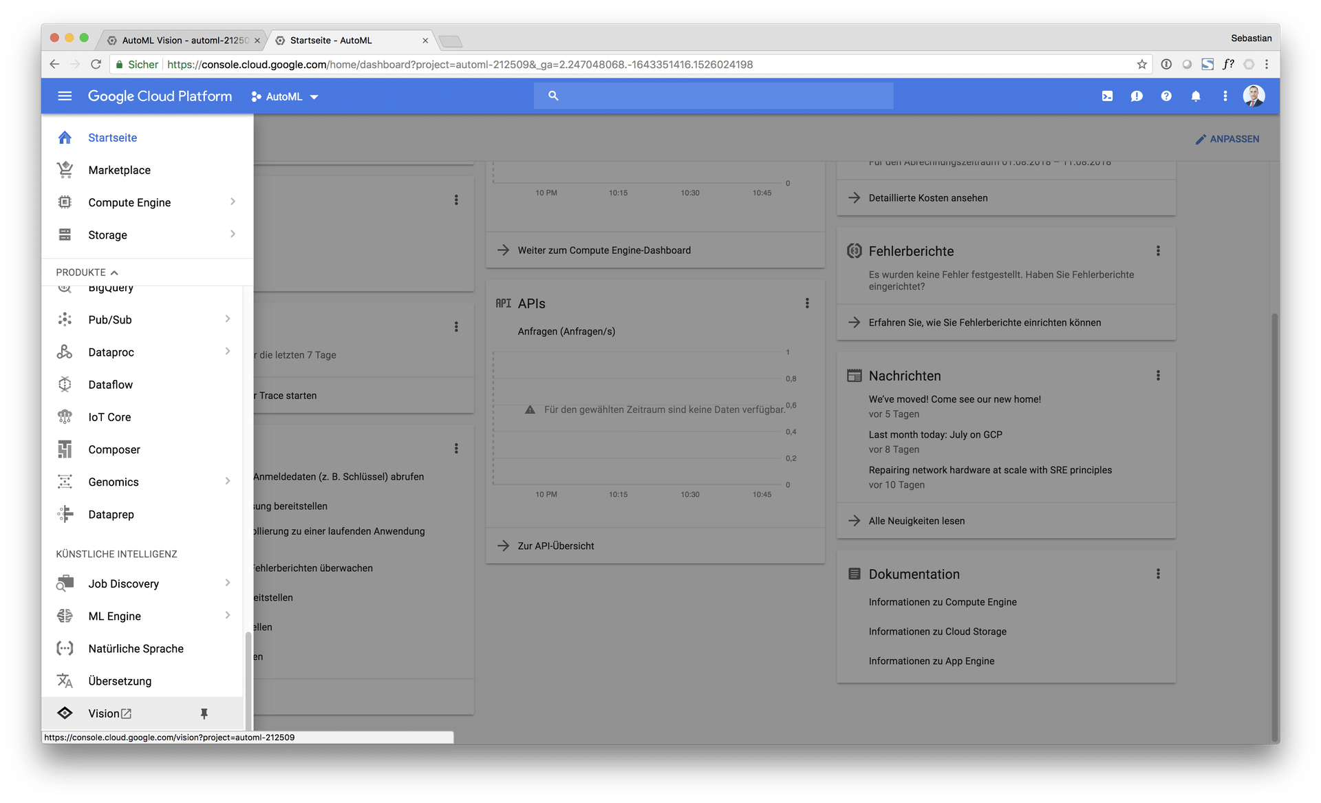
The start screen looks pretty unspectacular at this point. You can start by clicking on “Get started with AutoML” or read the documentation, which is pretty basic so far but informative, especially when you’re not familiar with basic machine learning concepts such as train-test-splits, overfitting, prcision / recall etc.
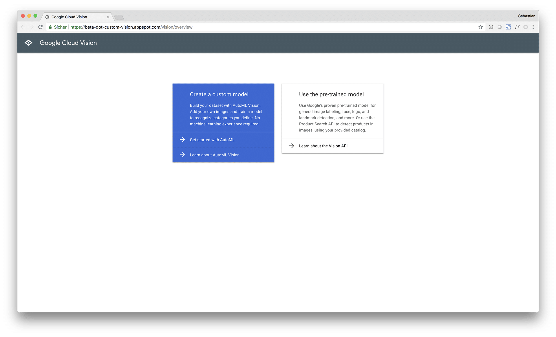
After you started, Google AutoML takes you to the dataset dialog, which is the first step on the road to the final AutoML model. So far, nothing to report here. Later, you will find here all of your imported datasets.
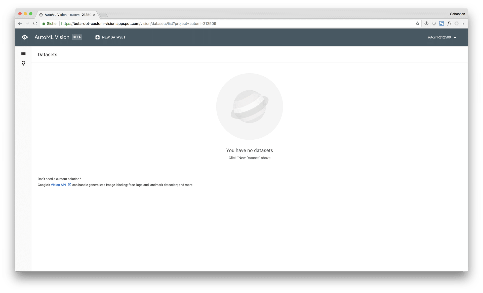
Generating the dataset
After hitting “+ NEW DATASET” AutoML takes you to the “Create dataset” dialog. As mentioned before, new datasets can be added using two different methods, shown in the next image.
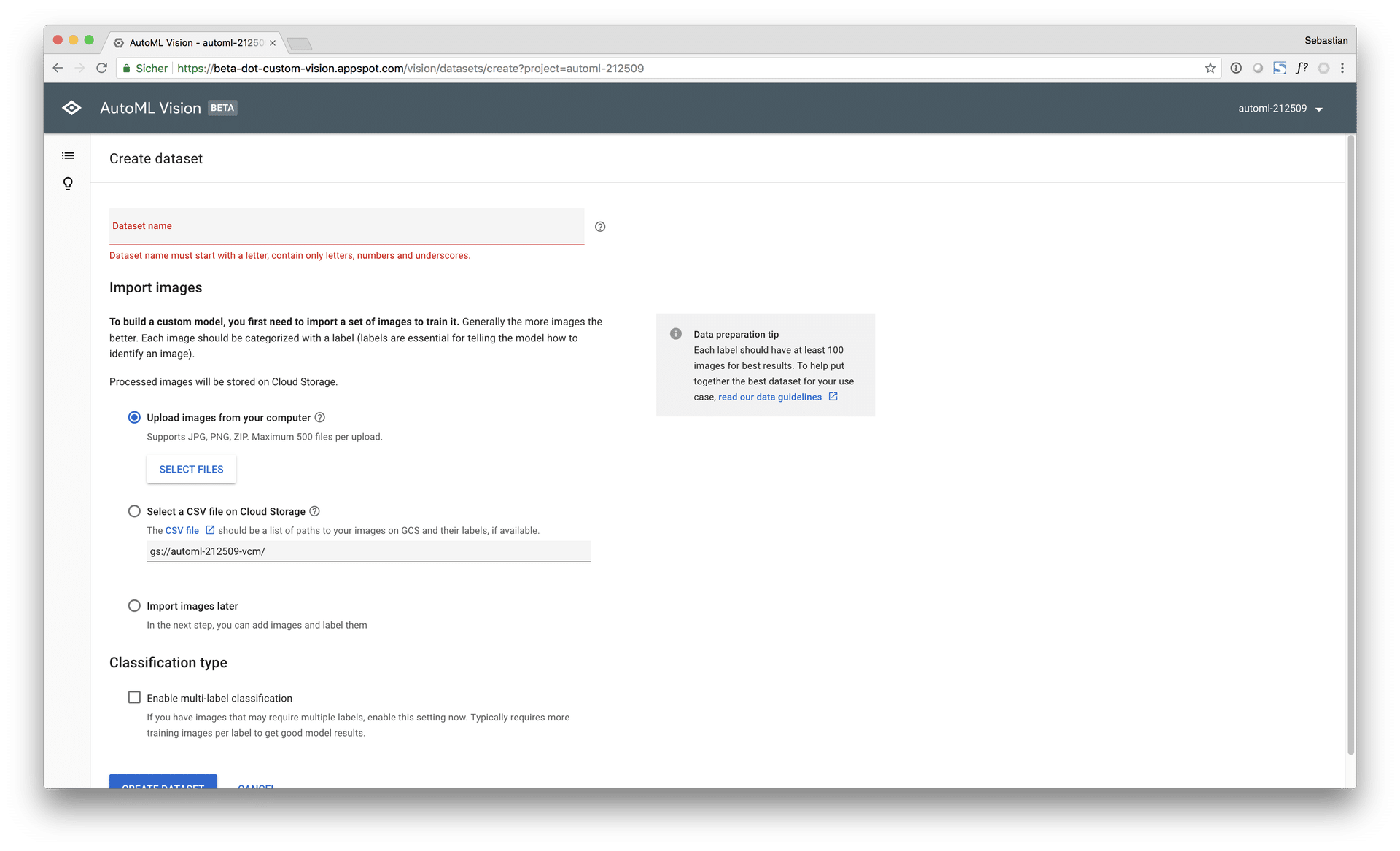
I’ve already uploaded the images from my computer as well as the CSV file containing the GS filepaths, partition information as well as the corresponding labels into the GS bucket. In order to add the dataset to AutoML Vision you must specify the filepath to the CSV file that contains the image GS-filepaths etc.
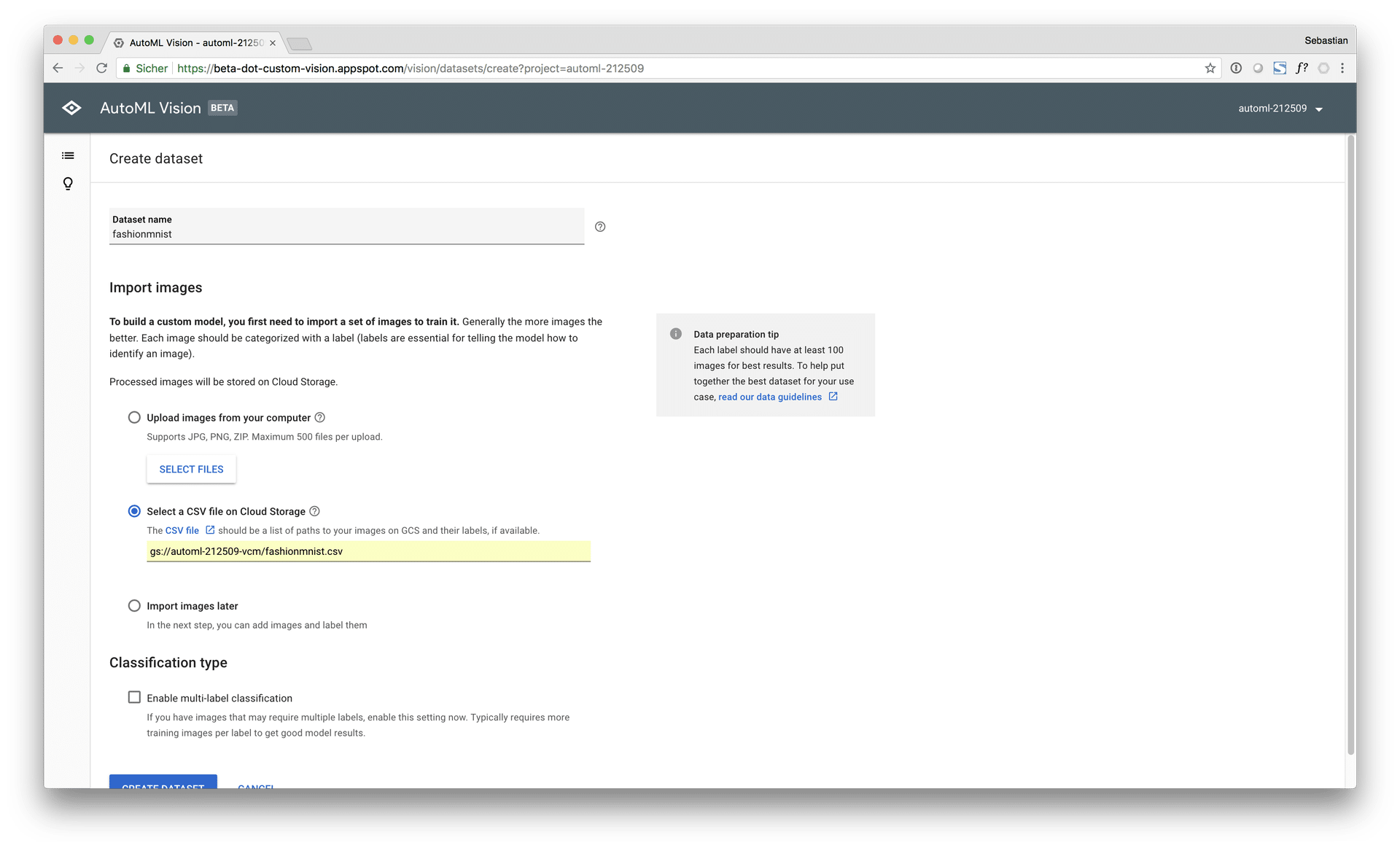
In the “Create dataset” dialog, you can also enable multi-label classification, if you have multiple labels per image, which is also a very helpful feature. After hitting “CREATE DATASET”, AutoML iterates over the provided file names and builds the dataset for modeling. What exactly is does, is neither visible nor documented. This import process may take a while, so it is showing you the funky “Knight Rider” progress bar.
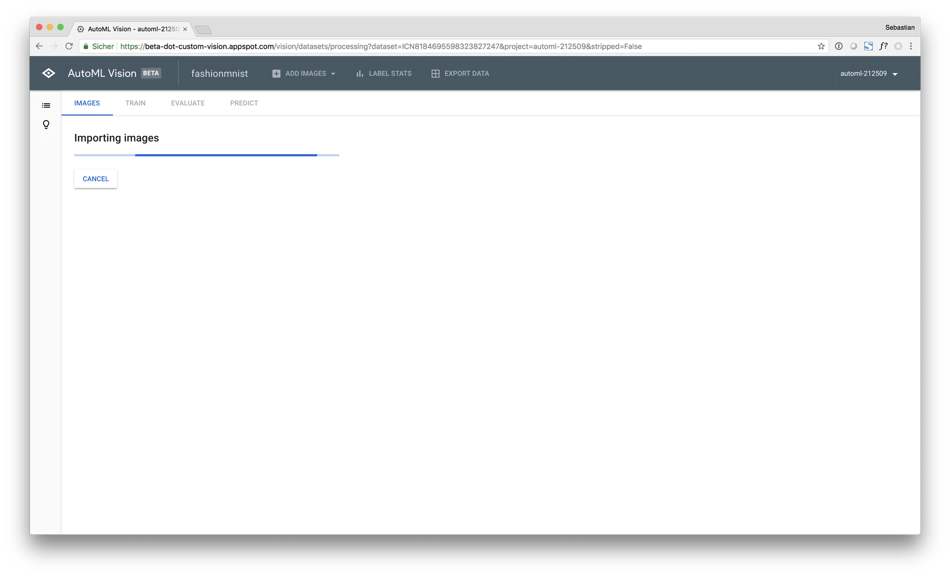
After the import is finished, you will recieve an email from GCP, informing you that the import of the dataset is completed. I find this helpful because you don’t have to keep the browser window open and stare at the progress bar all the time.
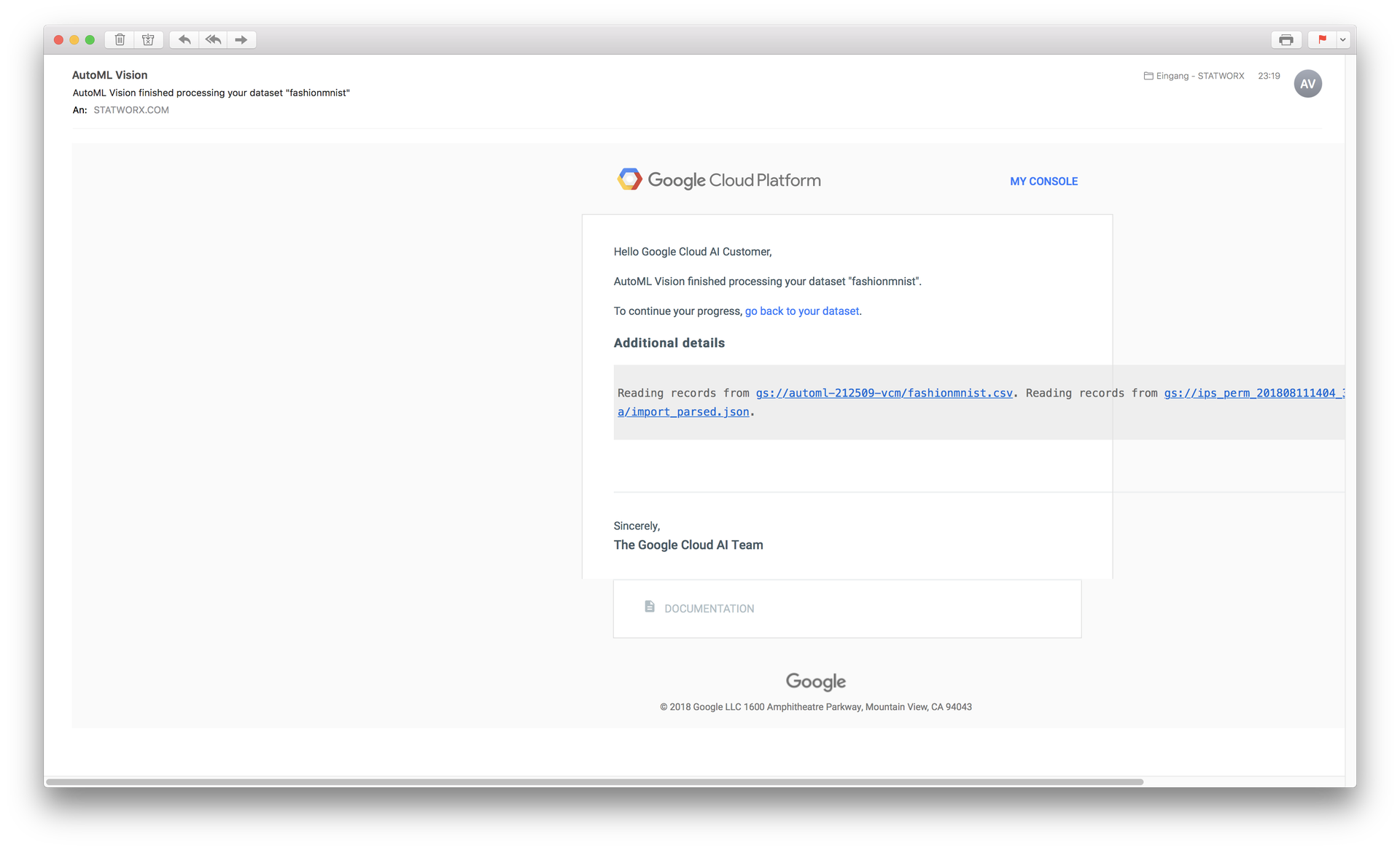
The email looks a bit weird, but hey, it’s still beta…
Training a model
Back to AutoML. The first thing you see after building your dataset are the imported images. In this example, the images are a bit pixelated because they are only 28×28 in resolution. You can navigate through the different labels using the nav bar on the left side and also manually add labels so far unlabeled images. Furthermore, you can request a human labeling service if you do not have any labels that come with your images. Additionally, you can create new labels if you need to add a category etc.
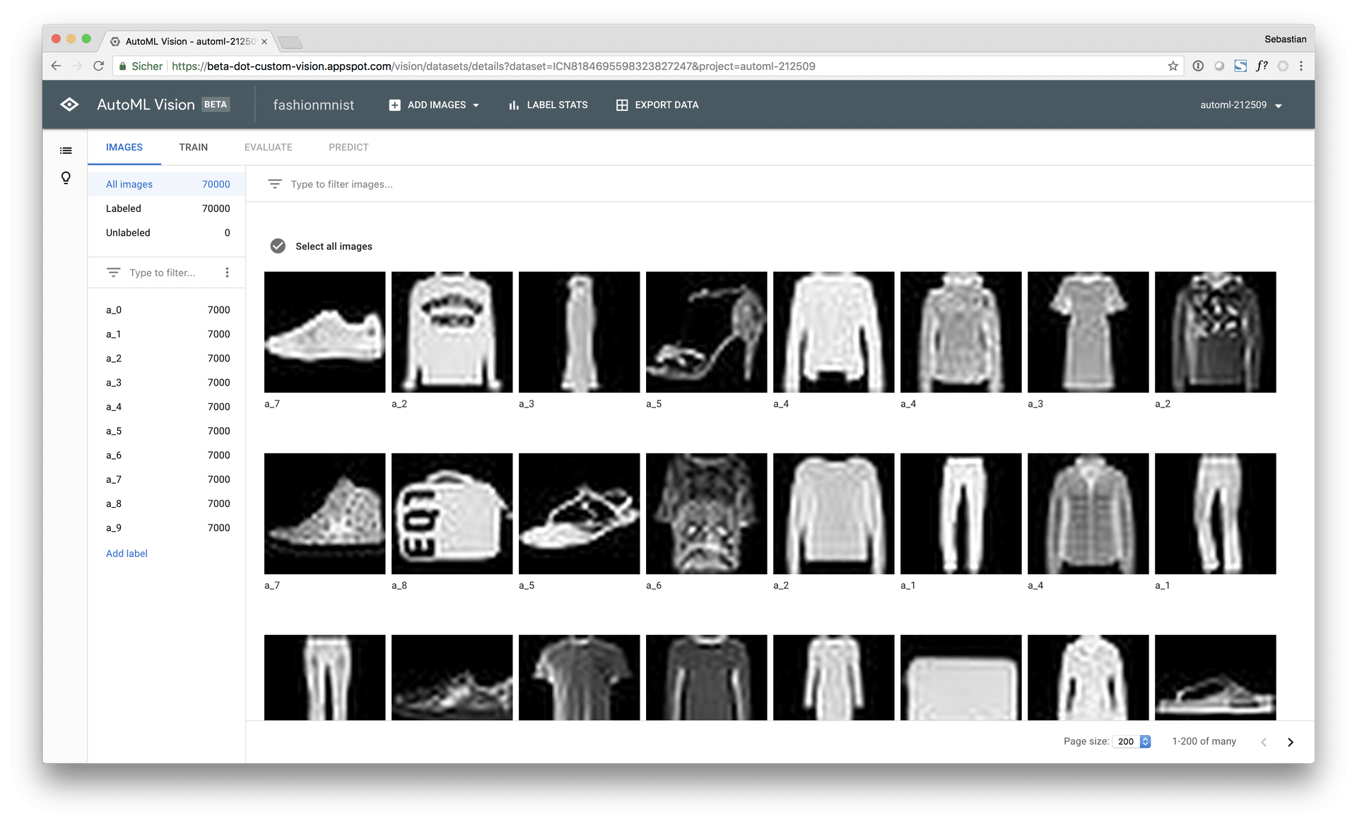
Now let’s get serious. After going to the “TRAIN” dialog, AutoML informs you about the frequency distribution of your labels. It recommends a minimum count of $n=100$ labels per class (which I find quite low). Also, it seems that it shows you the frequencies of the whole dataset (train, validation and test together). A grouped frquency plot by data partition would be more informative at this point, in my opinion.
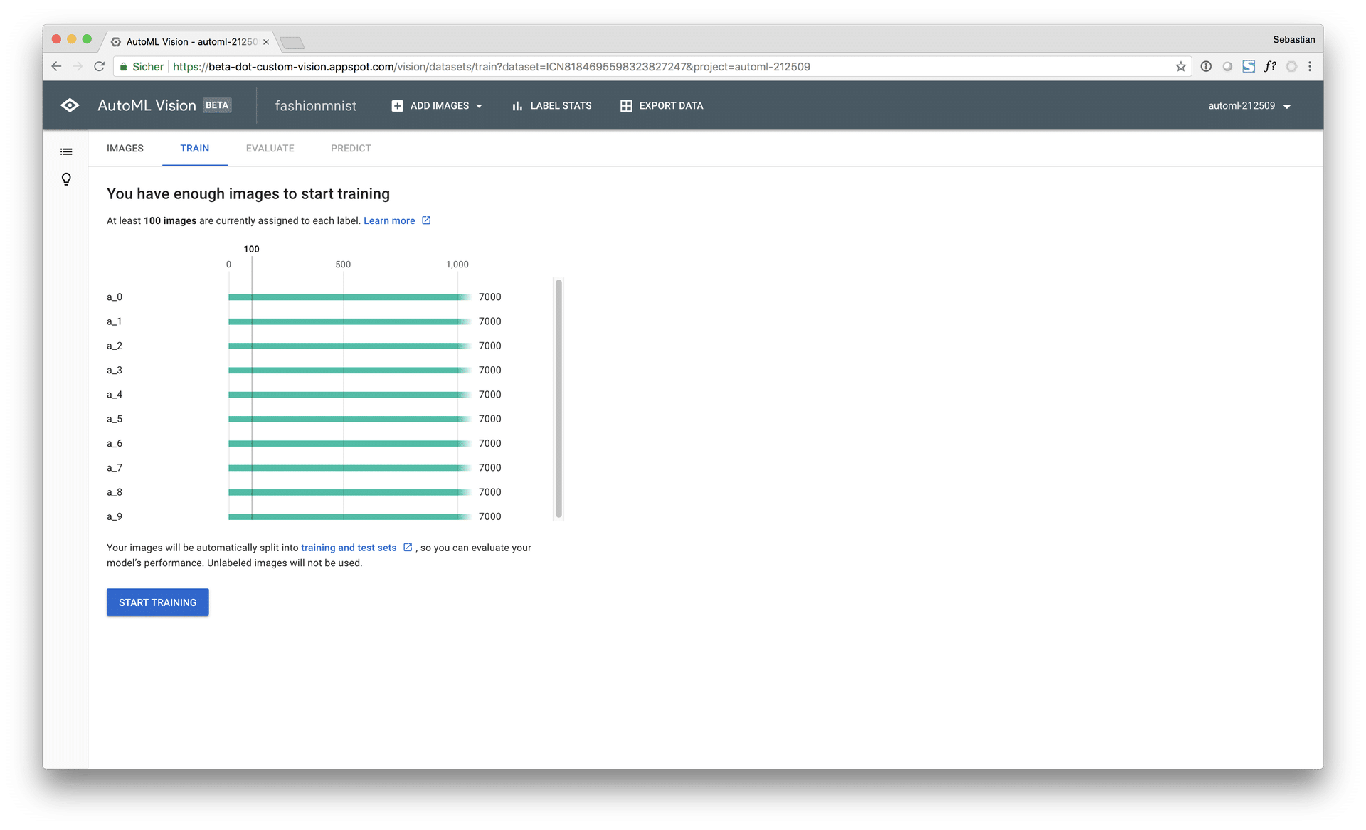
A click on “start training” takes you to a popup window where you can define the model name and the allocate a training budget (computing time / money) you are willing to invest. You have the choice between “1 compute hour”, whis is free for 10 models every month, or “24 compute hours (higher quality)” that comes with a price tag of approx. 480 $ (1 hour of AutoML computing costs 20 $. Hovever, if the architecture search converges at an earlier point, you will only pay the amount of computing time that has been consumed so far, which I find reasonable and fair. Lastly, there is also the option to define a custom training time, e.g. 5 hours.
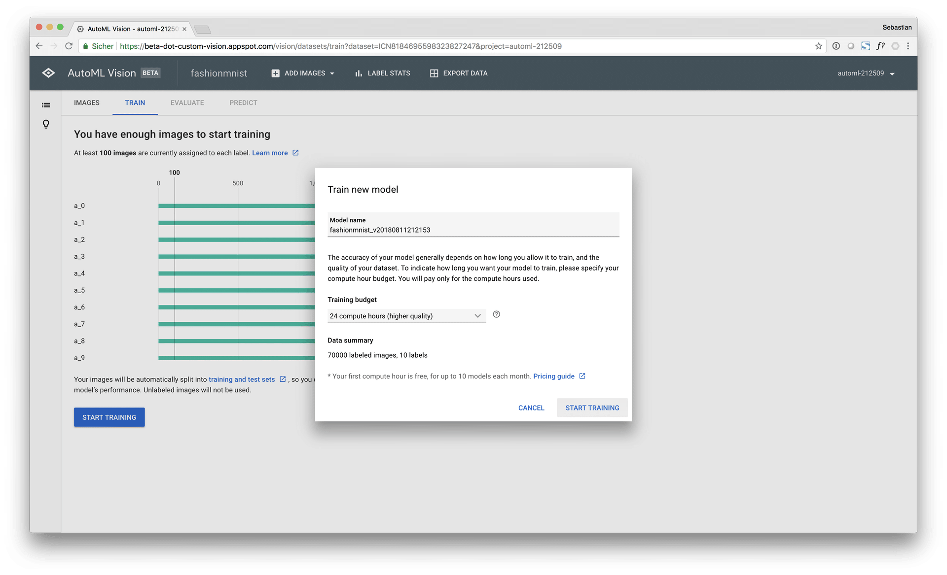
In this experiment, I tried both, the “free” version of AutoML but I also went “all-in” and seleced the 24 hours option to achieve the best model possible (“paid model”). Let’s see, what you can expect from a 480 $ cutting edge AutoML solution. After hitting “START TRAINING” the familiar Knight Rider screen appears telling you, that you can close the browser window and let AutoML do the rest. Naise.
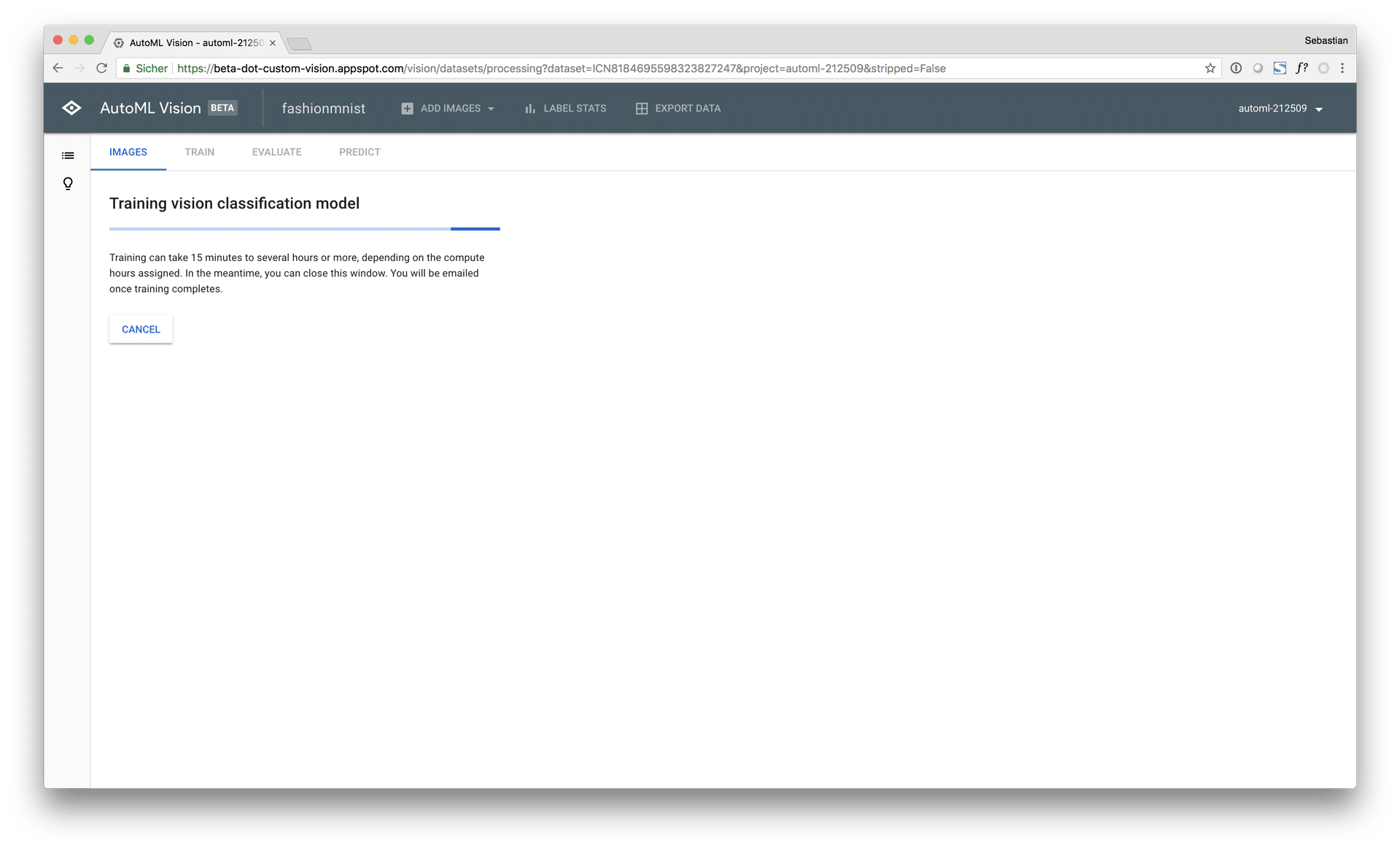
Results and evaluation
First, let’s start with the free model. It took approx. 30mins of training and seemed to have converged a solution very quickly. I am not sure, what exactly AutoML does when it evaluates convergence criteria but it seems to be different between the free and paid model, because the free model converged already around 30 minutes of computing and the paid model did not.
The overall model metrics of the free model look pretty decent. An average precision of 96.4% on the testset at a macro class 1 presision of 90.9% and a recall of 87.7%. The current accuracy benchmark on the Fashion-MNIST dataset is at 96.7% (WRN40-4 8.9M parameters) followed by 96.3% (WRN-28-10 + Random Erasing) while the accuracy of the low budget model is only at 89.0%. So the free AutoML model is pretty far away from the current Fashion-MNIST benchmark. Below, you’ll find the screenshot of the free model’s metrics.
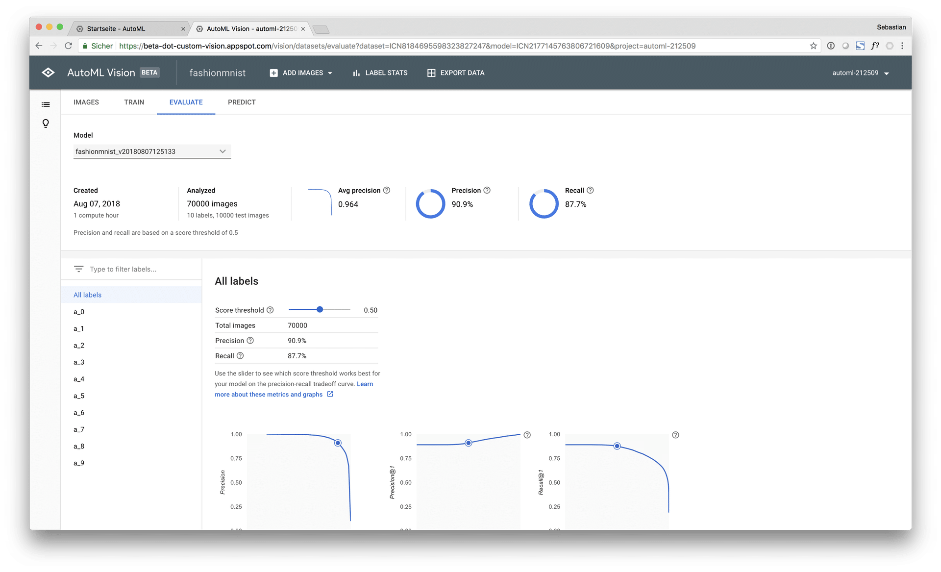
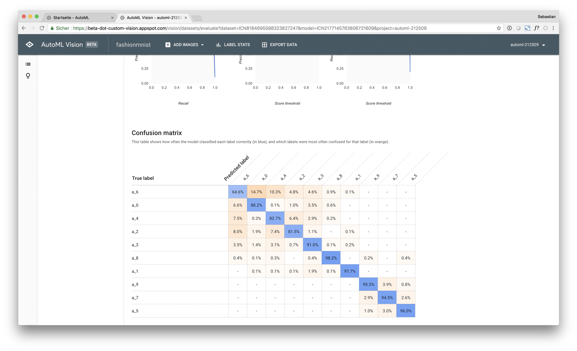
The model metrics of the paid model look significantly better. It achieved an average precision of 98.5% on the testset at a macro class 1 presision of 95.0% and a recall of 92.8% as well as an accuracy score of 93.9%. Those results are close to the current benchmark, however, not so close as I hoped. Below, you’ll find the screenshot of the paid model’s metrics.
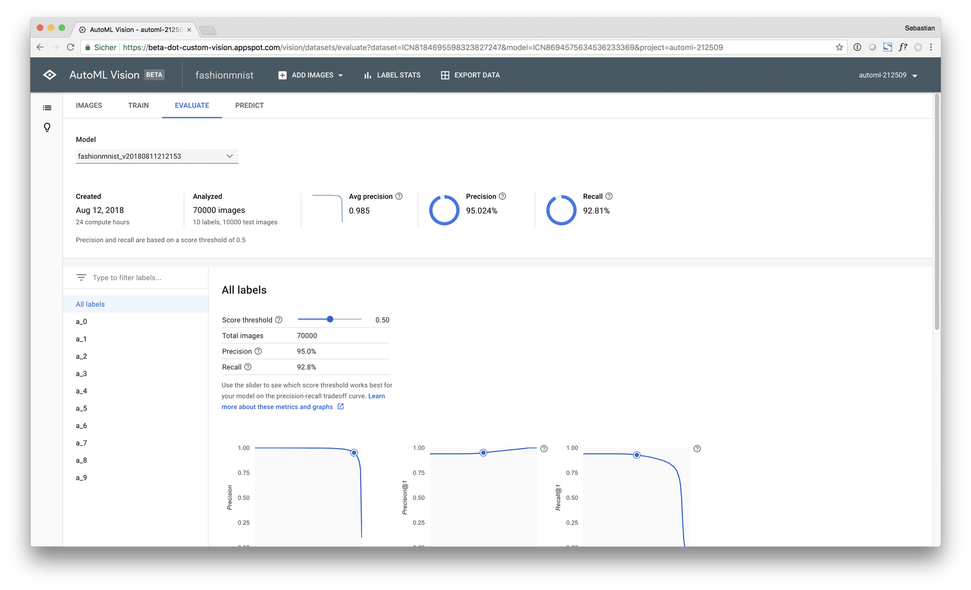
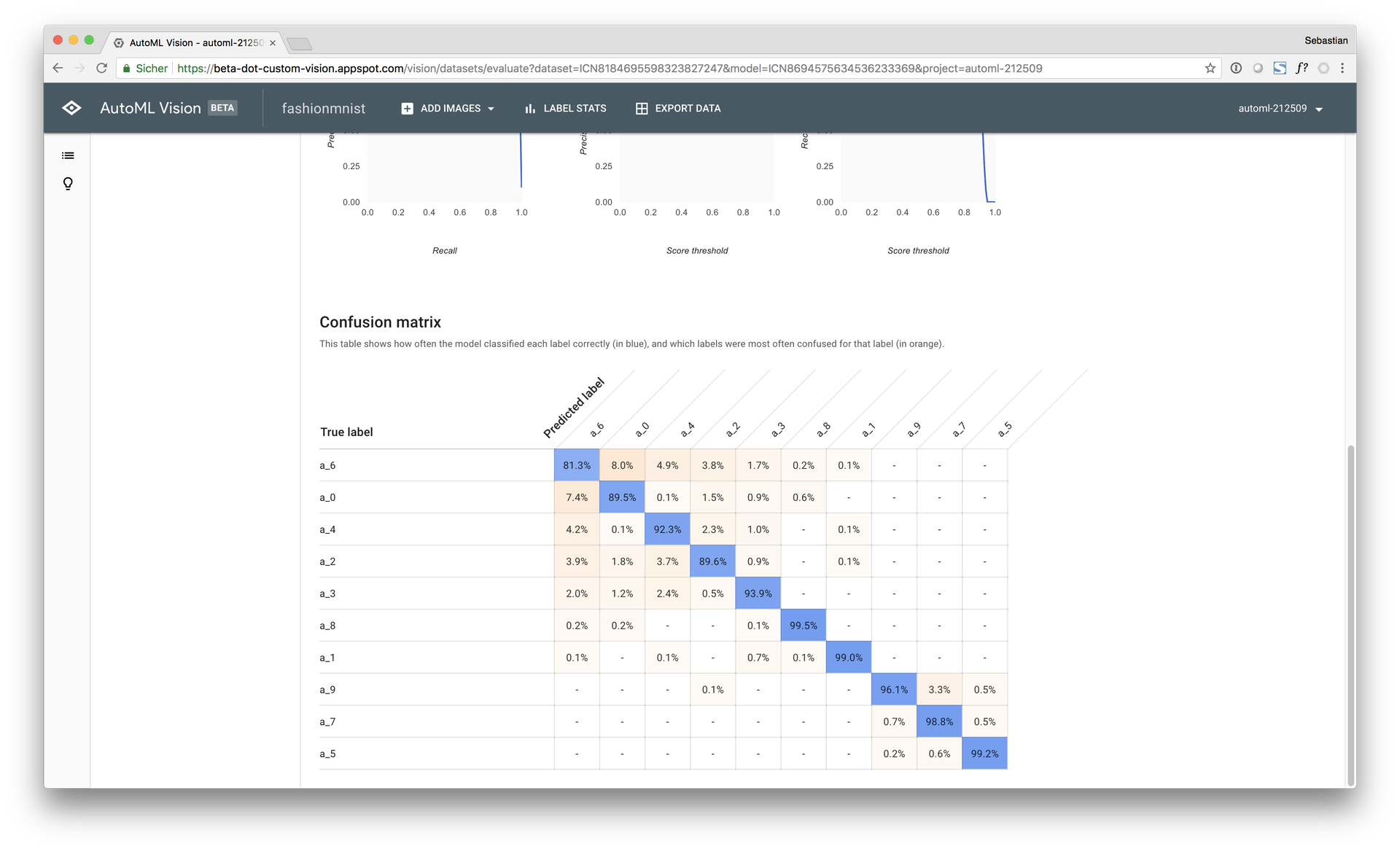
The “EVALUATE” tab also shows you further detailed metrics such as precision / recall curves as well as sliders for classification cutoffs that impact the model metrics respectively. At the bottom of the page you’ll find the confusion matrix with relative freuqencies of correct and misclassified examples. Furthermore, you can check images of false positives and negatives per class (which is very helpful, if you want to understand why and when your model is doing something wrong). Overall, the model evaluation functionalities are limited but user friendly. As a more profound user, of course, I would like to see more advanced features but considering the target group and the status of development I think it is pretty decent.
Prediction
After fitting and evaluating your model you can use several methods to predict new images. First, you can use the AutoML user interface to upload new images from your local machine. This is a great way for unexperienced users to apply their model to new images and get predictions. For advanced users and developers, AutoML vision exposes the model through an API on the GCP while taking care of all the technical infrastructure in the background. A simple Python script shows the basic usage of the API:
import sys
from google.cloud import automl_v1beta1


# Define client from service account json
client = automl_v1beta1.PredictionServiceClient.from_service_account_json(filename='automl-XXXXXX-d3d066fe6f8c.json')

# Endpoint
name = 'projects/automl-XXXXXX/locations/us-central1/models/ICNXXXXXX

# Import a single image
with open('image_10.jpg', 'rb') as ff:
    img = ff.read()

# Define payload
payload = {'image': {'image_bytes': img}}

# Prediction
request = client.predict(name=name, payload=payload, params={})
print(request)

# Console output
payload {
  classification {
    score: 0.9356002807617188
  }
  display_name: "a_0"
}
As a third method, it is also possible to curl the API in the command line, if you want to go full nerdcore. I think, the automated API exposure is a great feature because it lets you integrate your model in all kinds of scripts and applications. Furthermore, Google takes care of all the nitty-gritty things that come into play when you want to scale the model to hundrets or thousands of API requests simultaneously in a production environment.
Conclusion and outlook
In a nutshell, even the free model achieved pretty good results on the test set, given that the actual amount of time invested in the model was only a fraction of time it would have taken to build the model manually. The paid model achieved significantly better results, however at a cost note of 480 $. Obviously, the paid service is targeted at data science professionals and companies.
AutoML Vision is only a part of a set of new AutoML applications that come to the Google Cloud (check these announcements from Google Next 18), further shaping the positioning of the platform in the direction of machine learning and AI.
In my personal opinion, I am confident that automated machine learning solutions will continue to make their way into professional data science projects and applications. With automated machine learning, you can (1) build baseline models for benchmarking your custom solutions, (2) iterate use cases and data products faster and (3) get quicker to the point, when you actually start to make money with your data – in production.
faced the usual situation where we needed to transform a proof of concept (POC) into something that could be used in production. The “new” aspect of this transformation was that the POC was loaded with a tiny amount (a few hundred megabytes) but had to make ready for a waste amount of data (terabytes). The focus was to build pipelines of data which connect all the single pieces and automate the whole workflow from the database, ETL (Extract-Transform-Load) and calculations, to the actual application. Thus, the simple master-script which calls one script after another was not an option anymore. It was relatively clear that a program or a framework which uses DAG’s was necessary. So, within this post, I will swiftly go over what a DAG is in this context, what alternatives we considered and which one we have chosen in the end. Further, there will be a
What’s a DAG?
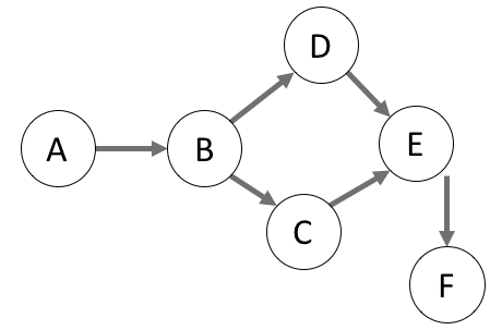
Directed Acyclic Graph
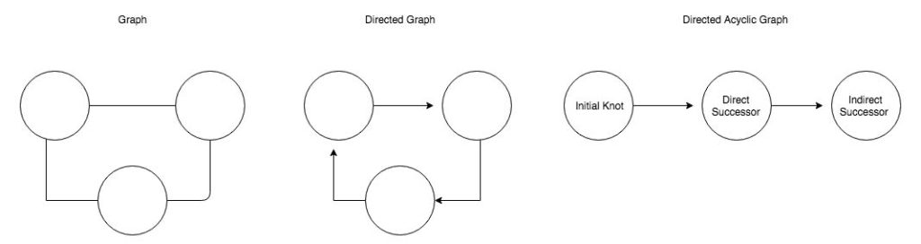
In programming, we can use this model and define every single task as a knot in the graph. Every job that can be done independently will be an initial knot with no predecessors and as such will have no relation point towards him. From there on we will link those tasks which are directly dependent on it. Continuing this process and connecting all task to the graph we can manifest a whole project into a visual guide. Even though this might be trivial for simple projects like ‘First do A then B and finally C’, once our workflow reaches a certain size or needs to be scalable, this won’t be the case anymore. Following this, it is advisable to express it in a DAG such that all the direct and indirect dependencies are expressed. This representation isn’t just a way to show the context visually such that non-technical people could grasp what is happening, but also gives a useful overview of all processes which could run concurrently, and which sequentially.
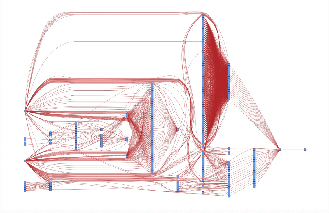
Just imagine if you have a workflow made up out of several dozen tasks (like the one above) some of which need to run sequentially and some that could run in parallel. Just imagine if one of these tasks failed without the DAG it wouldn’t be clear what should happen next. Which one needs to wait until the failed one finally succeed? Which can keep running since they do not depend on it? With a DAG this question can be answered quickly and doesn’t even come up if a program is keeping track of it. Due to this convenience, a lot of software and packages adopted this representation to automate workflows.
What were we looking for?
As mentioned, we were looking for a piece of software, a framework or at least a library as an orchestrator which works based on a DAG as we would need to keep track of the whole jobs manually otherwise – when does a task start, what if a task fails – what does it mean to the whole workflow. This is especially necessary as the flow needed to be executed every week and therefore monitoring it by hand would be tedious. Moreover, due to the weekly schedule an inbuilt or advanced scheduler would be a huge plus. Why Advanced? – There are simple schedulers like cron which are great for starting a specific job at a specific time but would not integrate with the workflow. So, one that also keeps track of the DAG would be great. Finally, it would also be required that we could extend the workflow easily. As it needed to be scalable it would be helpful if we could call a script – e.g., to clean data- several times just with a different argument – for different batches of data- as different nodes in the workflow without much overhead and code.
What were our options?
Once we settled on the decision that we need to implement an orchestrator which is based on a DAG, a wide variety of software, framework and packages popped up in the Google search. It was necessary to narrow down the amount of possibility so only a few were left which we could examine in depth. We needed something that was neither to heavily based on a GUI since it limits the flexibility and scalability. Nor should it be too code-intensive or in an inconvenient programming language since it could take long to pick it up and get everybody on board. So, options like Jenkins or WAF were thrown out right away. Eventually, we could narrow it down to three options:
Option 1 – Native Solution: Cloud-Orchestrator
Since the POC was deployed on a cloud, the first option was, therefore, rather obvious – we could use one of the cloud native orchestrators. They offered us a simple GUI to define our DAGs, a scheduler and were designed to pipe data like in our case. Even though this sounds good, the inevitable problem was that such GUIs are restricted, one would need to pay for the transactions, and there would be no fun at all without coding. Nevertheless, we kept the solution as a backup plan.
Option 2 – Apaches Hadoop Solutions: Oozie or Azkaban
Oozie and Azkaban are both open-source workflow manager written in Java and designed to integrate with Hadoop Systems. Therefore, they are both designed to execute DAGs, are scalable and have an integrated scheduler. While Oozie tries to offer high flexibility in exchange for usability, Azkaban has the tradeoff the other way around. As such, orchestration is only possible through the WebUI in the case of Azkaban. Oozie, on the other hand, relies on XML-Files or Bash to manage and schedule your work.
Option 3 – Pythonic Solution: Luigi or Airflow
Luigi and Airflow are both workflow managers written in Python and available as open-source frameworks.
Luigi was developed in 2011 by Spotify and was designed to be as general as possible – in contrast to Oozie or Azkaban which were intended for Hadoop. The main difference compared to the other two is that Luigi is code- rather than GUI-based. The executable workflows are all defined by Python code rather than in a user interface. Luigi’s WebUI offers high usabilitiy, like searching, filtering or monitoring the graphs and tasks.
Similar to this is Airflow which was developed by Airbnb and opened up in 2015. Moreover, it was accepted in the Apache Incubator since 2016. Like Luigi, it is also code-based with an interface to increase usability. Furthermore, it comes with an integrated scheduler so that one doesn’t need to rely on cron.
Our decision
Our first criterion for further filtering was that we wanted a code-based orchestrator. Even though interfaces are relatively straightforward to pick up and easy to get used to, it would come at the cost of slower development. Moreover, editing and extending would also be time-consuming if every single adjustment would require clicking instead of reusing function or code snippets. Therefore, we turned down option number one – the local Cloud-Orchestrator. The loss of flexibility shouldn’t be underestimated. Any learning or takeaways with an independent orchestrator could likely apply to any other project. This wouldn’t be the case for a native one, as it is bound to the specific environment.
The most significant difference between the other two options were the languages in which they operate. Luigi and Airflow are Python-based while Oozie and Azkaban are based on Java, and Bash scripts. Also, this decision was easy to determine, as Python is an excellent scripting language, easy to read, fast to learn and simple to write. With the aspect of flexibility and scalability in mind, Python offered us a better utility compared the (compiled) programming language Java. Moreover, the workflow definition needed to be either done in a GUI (again) or with XML. Thus, we could also exclude option two.
The last thing to settle was either to use Spotify’s Luigi or Airbnbs Airflow. It was a decision between taking the mature and stable or go with the young star of the workflow managers. Both projects are still maintained and highly active on GitHub with over several thousand commits, several hundred stars and several hundred of contributors. Nevertheless, there was one aspect which was mainly driving our decision – cron. Luigi can only schedule jobs with the usage of cron, unlike Airflow which has an integrated scheduler. But, what is actually the problem with cron?
Cron works fine if you want one job done at a specified time. However, once you want to schedule several jobs which depend on each other, it gets tricky. Cron does not regard these dependencies whether one task scheduled job needs to wait until the predecessor is finished. Let’s say we want a job to run every five minutes and transport some real-time data from a database. In case everything goes fine, we will not run into trouble. A job will start, it will finish, the next one starts and so on. However, what if the connection to the database isn’t working? Job one will start but never finishes. Five minutes later the second one will do the same while job one will still be active. This might continue until the whole machine is blocked by unfinished jobs or crashes. With Airflow, such a scenario could be easily avoided as it automatically stops starting new jobs when requirements are not met.
Summarizing our decision
We chose apache Airflow over the other alternatives base on:
-
No cron – With Airflow´s included scheduler we don’t need to rely on cron to schedule our DAG and only use one framework (not like Luigi).
-
Code Bases – In Airflow all workflows, dependencies, and schedulings are done in Python code. Therefore, it is rather easy to build complex structures and extend the flows.
-
Language – Python is a language somewhat natural to pick up and was available in our team.
Thus, Airflow fulfills all our needs. With it, we have an orchestrator which keeps track of the workflow we define by code using Python. Therefore, we could also easily extend the workflow in any directions – more data, more batches, more steps in the process or even on multiple machines concurrently won’t be a problem anymore. Further, Airflow also includes a nice visual interface of the workflows such that one could also easily monitor it. Finally, Airflow allows us to renounce crone as it comes with an advanced onboard scheduler. One that can not only start a task but also keeps track of each and is highly customizable in its execution properties.
In the
In the first part of this blog post, we talked about what a DAG is, how to apply this mathematical concept in project planning and programming and why we at
- DAG is short for directed acyclic graph and as such can represent relationships and dependencies
- This last aspect can be used in project management as it can become clear what task can run independently of each other and which can not
- The same properties can be used in programming, as software can determine which jobs can run concurrently or in which order the others have to finish (or fail).
Why did we choose Airflow:
- No Cron – With Airflow´s included scheduler we don’t need to rely on cron to schedule our DAGs and only use one framework (not like Luigi)
- Code Bases – In Airflow all the workflows, dependencies, and scheduling are done in Python code. Therefore, it is rather easy to build complex structures and extend the flows.
- Language – Python is a language somewhat natural to pick up, and that skill was already available in our team.
Preparation
The first thing was to set up a new virtual environment with Python and virtualenv.
$pip install virtualenv # if it hasn't been installed yet
$cd  # change into home

# create a separated folder with all environments
$mkdir env
$cd env
$virtualenv airflow
Once it has been created, we can source this environment whenever we want to work with Airflow, so we don’t get into conflict with other dependencies.
$source ~/env/airflow/bin/activate Then we can install all Python packages we will need
$ pip install -U pip setuptools wheel \
psycopg2\
Cython \
pytz \
pyOpenSSL \
ndg-httpsclient \
pyasn1 \
psutil \
apache-airflow[postgres]\
A Small Breeze
Once our setup is done, we can check if Airflow is correctly installed by typing airflow version
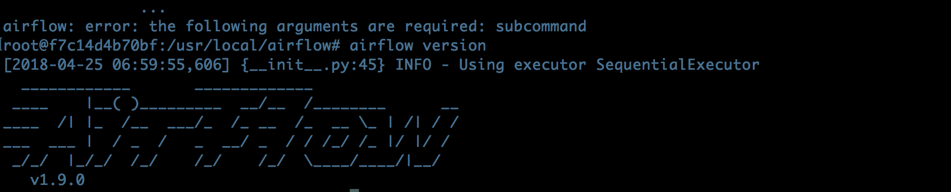
Initially, Airflow will run with a SQLite database, which cannot execute more than one task at a time and, therefore, should be switched out once you want or get serious about it. However, more on this later. Next, let us start with the typical hello world example. Navigate to your AIRFLOW_HOME-path which is by default a folder called airflow in your root directory. If you want to change this, edit the environment variable with export AIRFLOW_HOME=/your/new/path and call airflow version once again.
# ~/airflow/dags/HelloWorld.py

from airflow import DAG
from airflow.operators.dummy_operator import DummyOperator
from airflow.operators.python_operator import PythonOperator
from datetime import datetime, timedelta

def print_hello():
    return 'Hello world!'

dag = DAG('hello_world',
            description='Simple tutorial DAG',
            start_date= datetime.now() - timedelta(days= 4),
            schedule_interval= '0 12 * * *'
         )

dummy_operator= DummyOperator(task_id= 'dummy_task', retries= 3, dag= dag)

hello_operator= PythonOperator(task_id= 'hello_task', python_callable= print_hello, dag= dag)

dummy_operator >> hello_operator # same as  dummy_operator.set_downstream(hello_operator)
The first nine lines should be somewhat self-explanatory, just the import of the necessary libraries and the definition of the ‘hello world’-function. The interesting part starts at line ten. Here, we are going to define the core of our workflow, a DAG-Object with the identifier hello_world in this case and a small description what this workflow will be used for and what it does (line 10). As you might have suspected the argument, start_date defines the beginning date of the task. This date should always be in the past. Otherwise, the task would be triggered and always keep asking if it can run and as such it will remain active until it is planned. The schedule_interval define the periods when the graph should be executed. We either set with a cron-like notation as above or with some syntactical sugar Airflow offers. In the example above, we define that the task should run daily at 12:00 o’clock. The fact that it should run daily could have also been expressed with schedule_interval='@daily. The cron notation follows the schema minute - hour - day (of the month) - month - day (of the week), like mi h d m wd. With the usage of * as a wildcard, we gain the ability to schedule in very flexible intervals. Let’s say we want a job to run every first day of the month at twelve o’clock. In this case, we wouldn’t want a specific month nor a specific day of the week and as such replace the placeholder by wildcard * ( min h d * *). Since it should run at 12:00 we will replace mi with 0 and h with 12. Last but not least, we would plug in the day of the month as 1 and get our final cron-notation 0 12 1 * *. If we don’t want to be this specific but rather say run daily or hourly starting from the start_date, we could use Airflows sugar – @daily, @hourly, @monthly or @yeary.
Once we have this DAG-instance, we can start to fill it with some task. Instances of operators in Airflow represent these. Here, we initiate a DummyOperator and a PythonOperator. Both need to be assigned a unique id, but this time it only needs to be unique within the workflow. As the first operator, we define a DummyOperator which does nothing at all. We only want it to fill our graph and that we could test Airflow with a scenario as simple as possible. The second one is a PythonOperator. Additional to the assignment to a graph and the id, the operator requires a function which will be executed once the task is triggered. Now, we can use our hello_world function and attach it through the PythonOperator to our workflow.
Before we can finally execute our flow, we still need to set the relations between our tasks. This linking is done either with the binary operators << and >> or by calling the set_upstream and set_downstream methods, respectively. This way, we can set the dependency that first the DummyOperator needs to run and succeed before our PythonOperator is executed.
Now that our code is fine we should test it. Therefore, we should run it directly in the Python interpreter to check whether we have a syntax mistake. So, either run it in an IDE or the terminal with the command python hello_world.py. If the interpreter doesn’t throw an error – congratulation you didn’t screw up too bad. Next, we need to check if Airflow is aware of our DAG with airflow list_dags. Now, we should see our hello_world id in the printed list. If so, we can check whether each task is assigned to it with airflow list_task hello_world. Again, we should see some familiar ids namely dummy_task and hello_task. So far so good, seems like at least the assignment worked. Next up is a unit test of the individual operators with airflow test dummy_task 2018-01-01 and airflow test hello_task 2018-01-01. Hopefully, this doesn’t raise any error, and we can continue.
Now that we could deploy our example workflow we first need to initiate Airflow entirely. This requires three commands before we can continue to trigger our task manually.
airflow initdbto initiate the database where Airflow saves the workflows and their states:
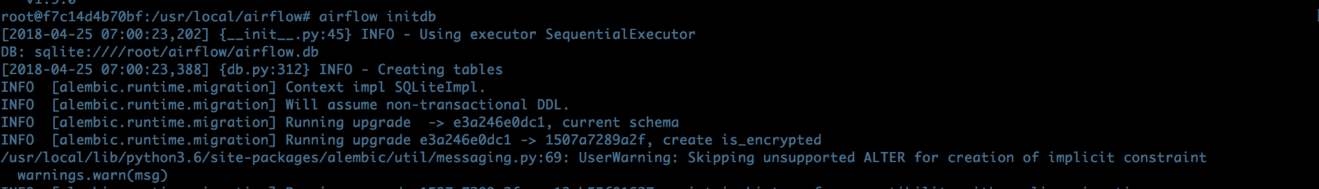
airflow webserverto start the web server atlocalhost:8080where we can reach the web interface:
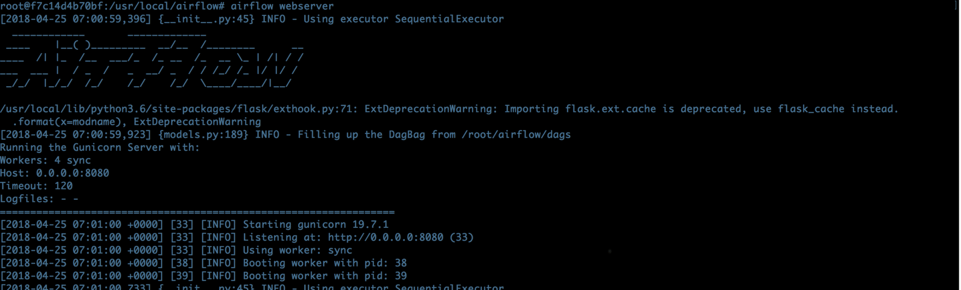
airflow schedulerto start the scheduling process of the DAGs such that the individual workflows can be triggered: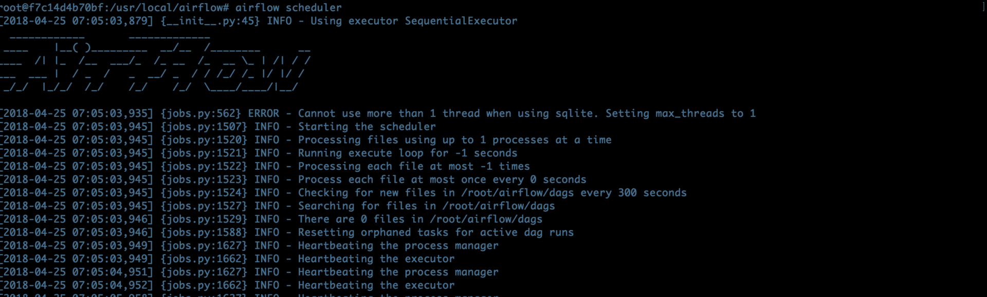
airflow trigger_dag hello_worldto trigger our workflow and place it on the schedule.
Now we can either open a web browser and navigate to the respective website or call open http://localhost:8080/admin/ in the terminal, and it should lead us to a web page like this.
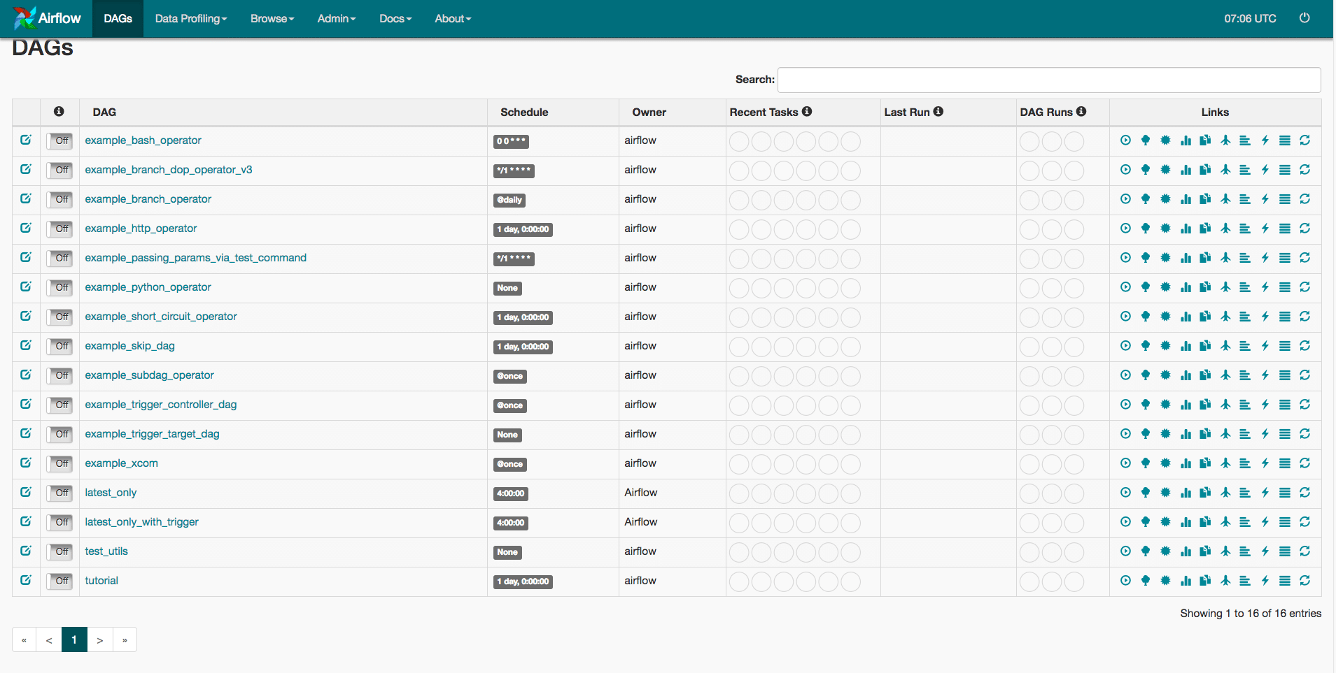
At the bottom, you should see your creation and the light green circle indicates that our flow is scheduled and running. The only thing left for us to do is to wait until it is executed. In the meantime, we can talk about the setup and how we could use some of the other executors.
The Backend
As mentioned before – once we want to get serious about the execution of our graphs we need to change the backend of Airflow. Initially, it will use a simple SQLite database which will limit Airflow only to execute one task at a time sequentially. Therefore, we will first change the connected database to PostgreSQL. In case you haven’t installed Postgres yet and need help with it I’d recommend you to check out its (wiki)[https://wiki.postgresql.org/wiki/Detailed_installation_guides]. I couldn’t possibly describe the process as good as the page. For those who are on a Linux-based system (sorry Windows), try sudo apt-get install postgresql-client or by using homebrew on a Mac – brew install postgresql. Another easy way would be to use a Docker container with the respective . Now, let us create a new database for Airflow by typing into to the terminal psql createdb airflow where all the metadata will be saved. Next, we need to edit the airflow.cfg file which should have appeared in your AIRFLOW_HOME folder (which is again by default airflow in your home directory) and restart the steps 1-4 from above (initdb…). Now, fire up your favorite editor and look for line 32 sql_alchemy_conn =. Here we are going to replace the SQLite connection string with the one from our PostgreSQL-Server and a new driver. This string will be made up out of postgresql+psycopg2://IPADRESS:PORT/DBNAME?user=USERNAME&password=PASSWORD
The first part tells sqlalchemy that the connection will lead to PostgreSQL and that it should use the psycopg2 driver to connect to it. In case you have Postgres locally installed (or in a container which maps to localhost) and did not change the standard port of 5432 our IPADRESS:PORT could be translated to localhost:5432 or simply localhost. The DBNAME would be changed to airflow in our case as we just created that for this purpose. The last two parts depend on what you have chosen as security measurements. Finally, we might have gotten a line that looks like this.
sql_alchemy_conn = postgresql+psycopg2://localhost/airflow?user=postgres&password=password Once we have done this, we can also change our executor in line 27 from executor = SequentialExecutor to an executor = LocalExecutor. That way every task will be started as a subprocess and as such the parallelizing will happen locally. This approach works great as long as our jobs are not too complicated or should run on multiple machines.
Once we reached that point, we need Celery as Executor. It is an asynchronous task/job queue based on distributed message passing. However, to use the CeleryExecutor, we need one more piece of software – a message broker. A message broker is an intermediary program module that translates a message from the ‘language’ of the sender to one for the receiver. The two most common options are either (redis)[https://redis.io/] or (rabbitmq)[https://www.rabbitmq.com/]. Use whatever you feel most comfortable with. Since we used rabbitmq, the whole process will continue with this broker but should be more or less analog for redis.
Again, for Linux and Mac users with homebrew, it is a one-liner to install it. Merely tip into your terminal sudo apt-get install rabbitmq-server or brew install rabbitmq and done. Next, we need a new user with a password and a virtual host. Both – user and host – can be created in the terminal by utilizing rabbitsmqs command line tool rabbitmqctl. Let’s say we want to create a new user called myuser with mypassword and a virtual host as myvhost. This can be achieved as follows:
$ rabbitmqctl add_user myuser mypassword
$ rabbitmqctl add_vhost myvhost
However, now back to the Airflows configuration. Navigate your editor to the line 230, and you will hopefully see broker_url =. This connection-string is similar to the one for the database and build with the pattern BROKER://USER:PASSWORD@IP:PORT/HOST. Our broker has the acronym amqp, and we can plug in our newly created user, password, and host. Unless you have changed the port or use a remote server your line should look something like this.
broker_url = amqp://myuser:mypassword@localhost:5672/myvhost Next, we need to grant Celery access to our airflow database and fill line 232 with db+postgresql://localhost:5432/airflow?user=postgres&password=password.
This string should be mostly equivalent to the one we used before. We only need to drop the driverpsycopg2 and instead add db+ at the beginning. And that’s it! All of the three executors should now be in your hand, and the setups are complete. Independent of the executor you have chosen, once you change the configuration you need to restart the steps 1-4 – initializing the DB, restart the scheduler and the web server. If you do this now, you will realize that the prompt changed slightly as it will show which executer you are using.
Conclusion
LocalExecutor for local multiprocessing. Moreover, due to Celery