Last time we dove deep into the world of a little salad bar just a few steps away from the STATWORX office. This time we are going to dig even deeper … well, we are going to dig a little deeper. Today’s Specials are cross-elasticities and the effect of promotions.
We talked so much about salads because the situation of our little island of semi-healthy lunch choices makes for an illustrative case on how we can calculate price elasticities – the measure generally agreed upon by economists to evaluate how any change in price affects demand. Since the intricacies of deriving these price elasticities of demand with regressions are to be the subject of this short blog series, the salad bar was a cheap example.
What we did so far
Specifically, in my last post, we wanted to know how a linear regression function relates to elasticity. It turns out that this depends on how the price and demand variables have been transformed. We explored four different transformations and in the end, we came to the conclusion that the log-log model fits our data best.
This was by no means an accident. Empirical explorations may occasionally guide us in choosing a different direction, but microeconomics arguments are heavily in favor of log-log models. The underlying demand curve describes demand most like economists assume it to behave. This model ensures that demand cannot sink below zero as the price increases; while on the other side, demand exponentially grows as the price decreases. Yet, the deductibility of a constant elasticity value is its most desirable feature. It makes the utilization of elasticity that much simpler.
Granted, if I’m being honest, the real reason the log-log model worked may have to do with the fact that I created the data. This salad vendor does exist, but obviously, they certainly did not fork over their sales data just because I thought their store would make an illustrative example. All the data we worked with was the result of how I imagined this little salad vendor’s market situation to be. Daily sales prices over the past two years were simulated for our little salad bar by randomly selecting prices between a certain price range, then a multiplicative demand function was used to derive sales with some added randomness. And with that, we were done simulating the data.
Obviously, this is far from the often messy historical data that one will encounter at retailers or any business that sells anything. There was no consideration of competition, no in-store alternatives, no new promotional activities, no seasonal effects, or any of the other business-specific factors that obscure price effects. The relationship between price and demand is usually obfuscated by the many other factors that influence a consumers’ buying decision. Thus, it is the intricacies of isolating the interfering factors that determine the success of empirical work.
A closer look at the data at hand
To illustrate this I went back to the sales data drawing board and made up some more data. For details, check out the code on our Github page. The results can be seen in the graph below. The graph actually consists of two graphs: a scatter plot that illustrates daily sales quantities over time and a line graph that also describes the price development over time. If one looks more closely at the graph, the development of sales cannot always be explained by just looking at the price. The second half of the year 2014 illustrates this most glaringly. In some cases, sales spikes occur which seem to be unrelated to the product price.

Additional information is thus needed. Obviously, there is a multitude of possible factors that might explain the discrepancies in the relationship between price and demand. And of course, when offered, we look at anything provided to us in order to evaluate whether we can extract some pricing-relevant insight from it. The two most desired requests concern information about promotional activities and intel on competitor prices. Luckily, we do not have to ask as I simulated the data and integrated it into the previously seen graph (see below). Promotional activities by the salad bar are indicated by thin blue lines across the two graphs and the pricing history of the closest competitor is illustrated in the graph below.
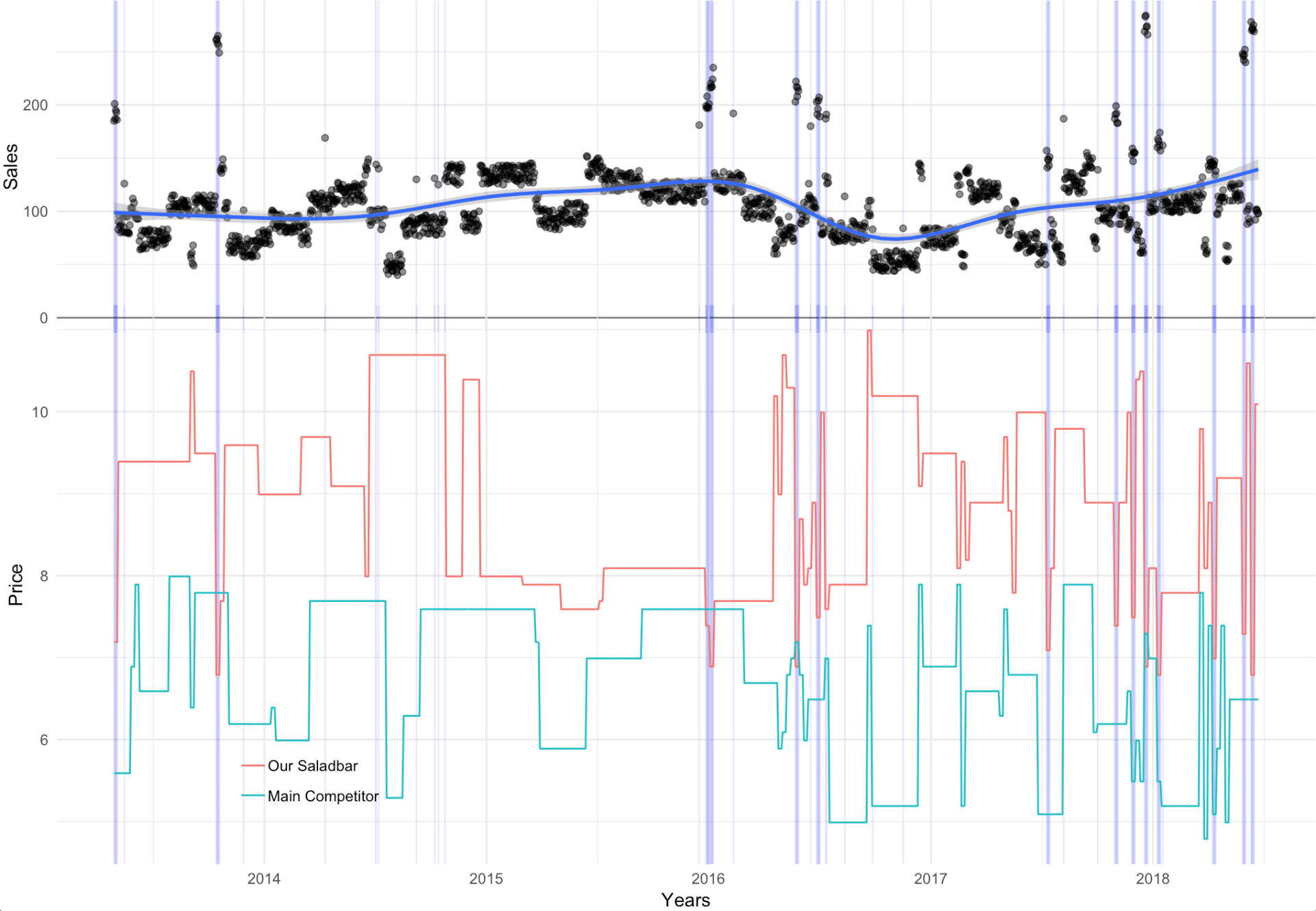
Almost surprisingly (though not really), the graph illustrates that both promotions and competitor prices impact the number of salads sold by our small salad bar. If we were now running the same log-log regression, the resulting elasticity score would be skewed.
But how does one include both the promotional data and the competitor price information? There are several fancy ways of doing it, but for now we’ll stick with simple (also often efficient) ways. For the promotional data, we will use a dummy variable – coded one for every day our salad bar turned on its promotions engine and zero otherwise. In reality though, the salad bar’s key promotional tools are an incentive-lacking stamp card and the occasional flyer with some time-limited coupons. The data describes the latter.
The theory of cross-price elasticity
To utilize the prices of competitors, we quickly need to delve into some economical theories. Next to the price elasticity of demand, there is a second concept called cross-price elasticity of demand. The two concepts are as similar, as their names suggest. Just look at the two formulas.
The formula for price elasticity:
![\[epsilon = frac{Delta qty/qty}{Delta price/price}\]](https://www.statworx.com/wp-content/ql-cache/quicklatex.com-a54b4a6166640946533bb725dcf213ac_l3.png "Rendered by QuickLaTeX.com")
And the formula for cross price elasticity:
![\[epsilon_{C} = frac{Delta qty/qty}{Delta price_{Comp}/price_{Comp}}\]](https://www.statworx.com/wp-content/ql-cache/quicklatex.com-5bbe228c7a4107822b98c3372686919e_l3.png "Rendered by QuickLaTeX.com")
The only thing that differs is the price with which one calculates. Instead of using the product’s price, one uses the competitor’s price. Conceptually, however price elasticity and cross-price elasticity slightly differ. With cross elasticity scores, it is plausible to get positive scores. However, with elasticity this is highly implausible and almost always indicates omitted variable bias, granted some luxury goods, like iPhones, may be the exception.
However, cross elasticities are actually commonly positive. The reason is captured by the terms substitutional goods and complementary goods. An obvious substitutional good would be a salad from the restaurant next to the salad bar. One eats either at the salad bar or at the restaurant. Thusly, a higher price for the salad at the restaurant could make it more likely that more customers choose to buy at the salad at our salad bar. A higher price at the restaurant would therefore consequently positively impact sales at the salad bar. The according cross elasticity score would be positive.
The influence of competitors
But we can also imagine negative cross elasticity scores. In this case, we are confronted with a complementary product. For example, next to our salad bar is a cute little coffee place. Coffee is perfect at overcoming the after-lunch food coma – so many people want one. Unfortunately, the greedy owner of this cute coffee shop just increased her prices – again! Annoying, but not a big problem for us, the restaurant with which our salad bar competes also sells cheap coffee. Now, this is a big problem for the salad bar. Their salad and the coffee from cute, but greedy shop are complementary products. As the coffee price increases, salad sales at our salad bar slow.
In Frankfurt, there are obviously only coffee shops with very reasonably priced coffee, so we stick to just the information about the main competitor. But how to operationalize the competitor price data? The conceptional and mathematical closeness between elasticity and cross elasticity suggests that one could treat them similarly. And indeed, it is a good starting point to include competitor prices the same way as the actual product prices, spoiler alert, logged.
| Advanced | Simple | |||
|---|---|---|---|---|
| Estimate | Std. Error | Estimate | Std. Error | |
| Intercept | 5.36 | 0.09 | 8.43 | 0.11 |
| Log Price | -1.45 | 0.03 | -1.76 | 0.05 |
| Promo | 0.45 | 0.02 | ||
Log Price |
1.23 | 0.03 | ||
Adjusted  |
0.80 | 0.41 | ||
Let’s look at the output in the table above. As I was in full control of the data generation process – and since we know what the underlying elasticity actually was – I set it at -1.5. Obviously, because of the minuscule level of randomness added, both models do reasonably well. Even withstanding and the standard errors, there is still a clear winner. By ignoring the impact of promotional activities and the competitor’s prices, the price elasticity estimate of the simpler model is biased. Here the difference is relatively small, but with real data, the difference can be substantial or as we omit essential information here systemic.
That is all! In the next blog post in this series, we introduce more complex relationships between price, promotions, competitor pricing, and concepts to utilize the insights for business purposes.